Hydrogen molecule †In this tutorial, how to execute pw.x and how to converge computational parameters, such as kinetic energy cutoff and box size are described by taking hydrogen molecule (H2) as an example.
How to optimize the molecular geometry is also described. In a standard plane-wave pseudopotential code, three-dimensional periodic boundary condition is employed, and an isolated molecule is modeled by placing it in a large box in such a way that the electrostatic interactions with neighboring images can be negligible. If the box is large enough, the Brillouin zone becomes small (as it scales as (2p/a)**3), thus the Brillouin zone is sampled only at the Gamma point [(0,0,0)]. In this case, the accuracy of the calculation is controlled by increasing the kinetic energy cutoff, which corresponds to increasing the real-space mesh (resolution of the wave function in real space) and by increasing the box size. The latter is to confirm that the interaction between image molecules is negligibly small and that the model mimics the molecule in its an isolated state. Preliminary †SCF calculation †Let us begin with an SCF calculation of H2 having the experimental bond length of 0.74 Angstrom in a cubic box with the edges of 10 Angstrom. We use the SG15 optimized norm-conserving pseudopotentials with the cutoff energy of 30 Ry. The input file for this calculation is called "h2_scf.in" and is the following: &control calculation = 'scf' restart_mode = 'from_scratch', pseudo_dir = '/home/ikutaro/QE/pseudo/' outdir = './tmp/' prefix = 'h2' tprnfor = .true. forc_conv_thr = 1.d-4 / &system ibrav = 1 A = 10.d0 nat = 2 ntyp = 1 nbnd = 4 ecutwfc = 30.0 ecutrho = 120.0 / &electrons diagonalization = 'david' conv_thr = 1.0e-12 mixing_beta = 0.1 / ATOMIC_SPECIES H 0.0000 H_ONCV_PBE-1.0.upf ATOMIC_POSITIONS (angstrom) H 0.000000000000 0.000000000000 0.00000000000 H 0.000000000000 0.000000000000 0.74000000000 K_POINTS (gamma) Here the number of electron is 2 and thus the minimum number of bands is 1, but slightly large number of bands of 4 is used. Note "pseudo_dir" and "outdir" should be modified according to the environment. To perform the SCF calculation, we use pw.x. Here let us assume we are going to use pw.x in $HOME/QE/src/qe-6.6 and execute the following $ mpirun -np 2 $HOME/QE/src/qe-6.6/bin/pw.x < h2_scf.in > h2_scf.out or for the group's cluster execute $ qsub h2.sh where the job script "h2.sh" looks like #$ -S /bin/bash
#$ -cwd
#$ -q xe1.q
#$ -pe x8 8
#$ -N H2
#
module load intel/2020.2.254
module load intelmpi/2020.2.254
#
INPUT_FILE='h2_scf.in'
OUTPUT_FILE='h2_scf.out'
#
PW_DIR=/home/ikutaro/QE/src/qe-6.6/bin
#
MPI_COMMAND=mpirun
PW_COMMAND=pw.x
PW=$PW_DIR/$PW_COMMAND
#
I_MPI_PIN=1
I_MPI_FABRICS=shm:ofa
OMP_NUM_THREADS=1
#
cat $PE_HOSTFILE | awk '{ print $1":"$2/ENVIRON["OMP_NUM_THREADS"] }' >
hostfile.$JOB_ID
#
$MPI_COMMAND $PW < $INPUT_FILE > $OUTPUT_FILE
When the calculation starts, you can see the following header in the output file (h2_scf.out) as Program PWSCF v.6.6 starts on 20Jan2021 at 10:38:59
This program is part of the open-source Quantum ESPRESSO suite
for quantum simulation of materials; please cite
"P. Giannozzi et al., J. Phys.:Condens. Matter 21 395502 (2009);
"P. Giannozzi et al., J. Phys.:Condens. Matter 29 465901 (2017);
URL http://www.quantum-espresso.org",
in publications or presentations arising from this work. More details at
http://www.quantum-espresso.org/quote
When the SCF convergence is archived, the following can be found in the output file (h2_scf.out). ! total energy = -2.31431570 Ry
estimated scf accuracy < 5.3E-13 Ry
The total energy is the sum of the following terms:
one-electron contribution = -3.79278260 Ry
hartree contribution = 2.01958267 Ry
xc contribution = -1.37197485 Ry
ewald contribution = 0.83085908 Ry
convergence has been achieved in 15 iterations
If "tprnfor = .true." the following lines can also be found Forces acting on atoms (cartesian axes, Ry/au):
atom 1 type 1 force = 0.00000000 0.00000000 -0.03012711
atom 2 type 1 force = 0.00000000 0.00000000 0.03012711
Total force = 0.042606 Total SCF correction = 0.000000
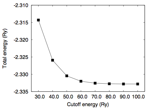
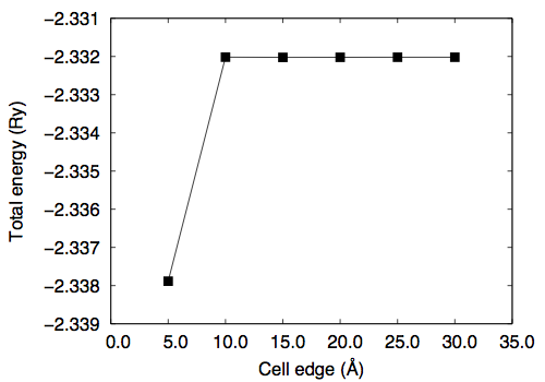
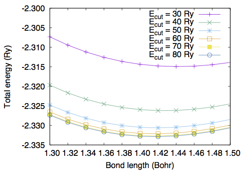
Use the "less" or "more" command to see the file. Convergence study †Convergence wrt cutoff †To study the convergence of the total energy, we calculate the total energy as a function of kinetic energy cutoff ("ecutwfc") by fixing the molecular structure. Note that in the present case normconserving pseudopotential is used and ecutrho is fixed to 4 times larger than ecutwfc (ecutrho = 4 * ecutwfc). Use h2_scf_ecutwfc*.in. Results are as follows # ecutwfc (Ry) total energy (Ry) 30.0 -2.31431279 40.0 -2.32593152 50.0 -2.33045981 60.0 -2.33201780 70.0 -2.33257560 80.0 -2.33275476 90.0 -2.33280832 100.0 -2.33281717 Convergence wrt box size †Then let us calculate the total energy as a function of the cell edge. In this study, ecutwfc=60.0 Ry is used. Create your own input file by copying one of the input file from previous calculations. # a (Angstrom) total energy (Ry) 5.0 -2.33788501 10.0 -2.33201780 15.0 -2.33202479 20.0 -2.33202183 25.0 -2.33202063 30.0 -2.33202053 Optimizing the bond length (1) †Let us determine the bond length of H2. First, we calculate the total energy as a function of bond length. The input files are the same as the one for the SCF calculation, but the position of the second H atom. We set the z-coordinate of the second H atom ranging from 1.3 to 1.5 Bohr. Use h2_scf_ecutwfc60_d*.in. Here is the result with ecutwfc=60Ry : 1.30 -2.32657183 1.32 -2.32840377 1.34 -2.32984183 1.36 -2.33091143 1.38 -2.33163627 1.40 -2.33203866 1.42 -2.33213950 1.44 -2.33195843 1.46 -2.33151384 1.48 -2.33082299 1.50 -2.32990212 By fitting the total energy to 6th-order polynomial, the equilibrium bond length of 1.4169 Bohr is obtained. Optimizing the bond length (2) †Alternatively, one can optimize the geometry (internal coordinate) by using the Hellmann-Feynman forces. The input file is as follows. Let's name it 'h2_relax.in.' Here we use the convergence threshold for the forces of 1.0 x 10⁻⁴ Ry/Bohr. &control calculation = 'relax' restart_mode = 'from_scratch', pseudo_dir = '/home/ikutaro/QE/pseudo/' outdir = './tmp/' prefix = 'h2' tprnfor = .true. forc_conv_thr = 1.d-4 / &system ibrav = 1 A = 10.d0 nat = 2 ntyp = 1 nbnd = 4 ecutwfc = 30.0 ecutrho = 120.0 / &electrons diagonalization = 'david' conv_thr = 1.0e-12 mixing_beta = 0.1 / &ions ion_dynamics = 'bfgs' / ATOMIC_SPECIES H 0.0000 H_ONCV_PBE-1.0.upf ATOMIC_POSITIONS (angstrom) H 0.000000000000 0.000000000000 0.00000000000 H 0.000000000000 0.000000000000 0.74000000000 K_POINTS (gamma) The main differences from the SCF calculation are calculation = 'relax' and &ions ion_dynamics='bfgs' / Here we use the BFGS algorithm for the structural optimization. Note the namelist &ions should be given even though the default parameters are used. In such a case &ions / can be used. When the convergence for the structural relaxation is achieved, following message can be found in the output as: bfgs converged in 4 scf cycles and 3 bfgs steps
(criteria: energy < 1.0E-04 Ry, force < 1.0E-04 Ry/Bohr)
End of BFGS Geometry Optimization
and the final coordinates follow as: Begin final coordinates ATOMIC_POSITIONS (angstrom) H 0.0000000000 0.0000000000 -0.0113658051 H 0.0000000000 0.0000000000 0.7513658051 End final coordinates The bond length of 1.4169 Bohr (0.750 Angstrom) obtained by the structural optimization by using the Hellmann-Feynman forces is in good agreement with that obtained by the manual structural optimization. Exercise †The bond length also depends on the computational parameters such as cutoff energy and box size. Calculate the bond length as a function of cutoff energy and estimate the converged bond length. |
![[PukiWiki] [PukiWiki]](image/logo_state-senri3_80x80.png)


