- バックアップ一覧
- 差分 を表示
- 現在との差分 を表示
- ソース を表示
- QE_tutorial/Au へ行く。
Gold †
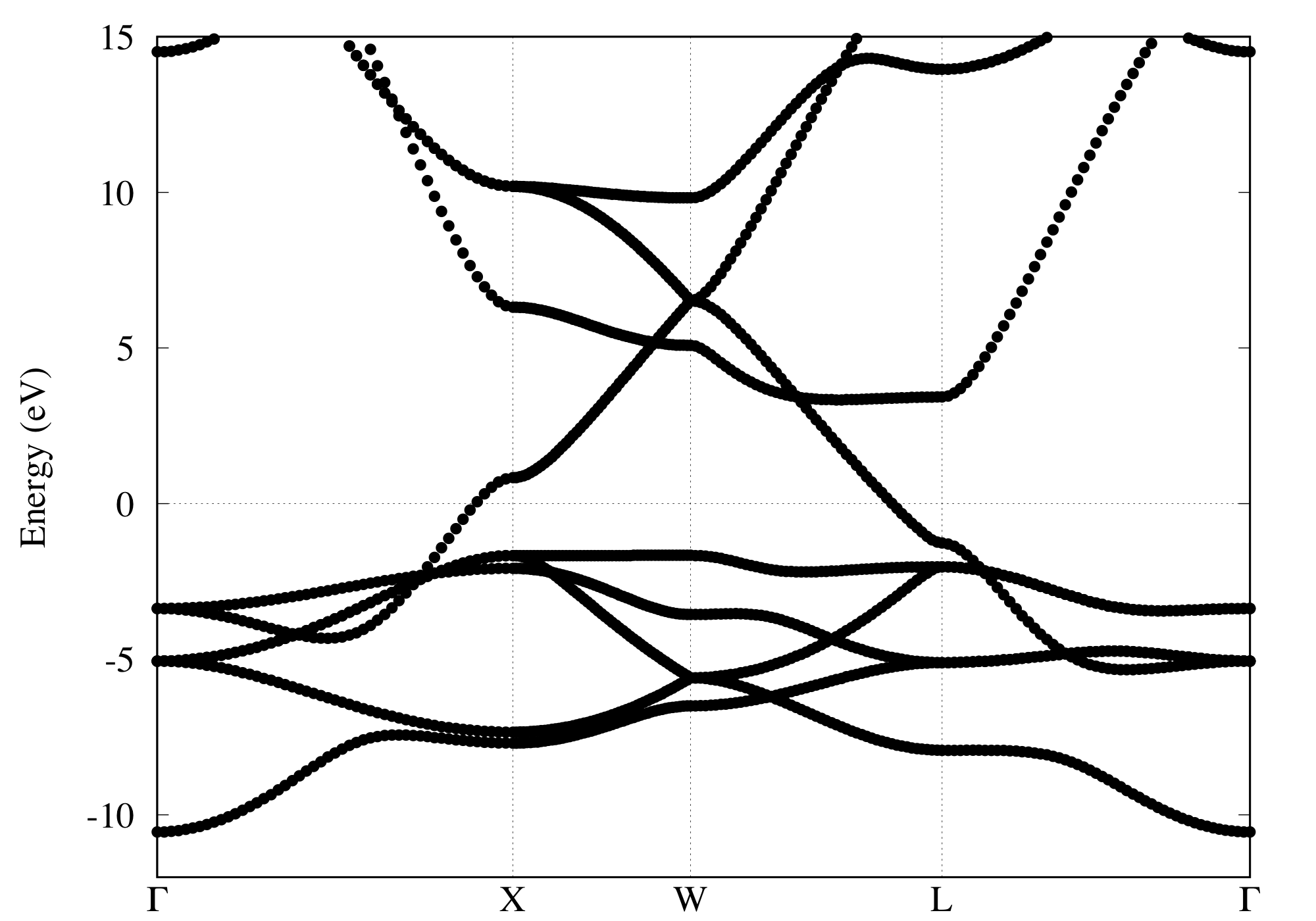
In this tutorial how to draw a band structure is described by taking gold (Au) in the face centered cubic structure as an example
SCF calculation †
First, perform an SCF calculation to get the charge density.
- Input file: au_scf.in
&control
   calculation='scf'
   restart_mode='from_scratch',
   pseudo_dir = '/home/ikutaro/QE/pseudo/'
   outdir='./tmp'
   prefix='au'
   tprnfor = .true.
   tstress = .true.
   forc_conv_thr = 1.d-4
   nstep=10000
/
&system
   ibrav = 2
   A     = 4.00
   !A     = 4.079
   nat   = 1
   ntyp  = 1
   ecutwfc = 40.0
   ecutrho = 400.0
   occupations='smearing'
   smearing='mp'
   degauss=0.01
   nbnd=24
   !input_dft='vdW-DF2-B86R'
   !assume_isolated = 'esm', esm_bc='bc1'
/
&electrons
   diagonalization='cg'
   conv_thr = 1.0e-12
   mixing_beta = 0.1
/
&ions
 ion_dynamics='bfgs'
/
&cell
 cell_dynamics='bfgs'
/
ATOMIC_SPECIES
 Au 0.0000 au_pbe_v1.uspp.F.UPF
ATOMIC_POSITIONS (crystal)
Au      0.000000000000      0.000000000000      0.00000000000
K_POINTS (automatic)
16 16 16 0 0 0
- Execution
mpirun -np 8 < au_scf.in > au_scf.out
Cell optimization †
For the cell optimization, use the input file like follows
- Input file: au_vc-relax.in
&control
   calculation='vc-relax'
   restart_mode='from_scratch',
   pseudo_dir = '/home/ikutaro/QE/pseudo/'
   outdir='./tmp'
   prefix='au'
   tprnfor = .true.
   tstress = .true.
   forc_conv_thr = 1.d-4
   nstep=10000
/
&system
   ibrav = 2
   A     = 4.00
   !A     = 4.079
   nat   = 1
   ntyp  = 1
   ecutwfc = 40.0
   ecutrho = 400.0
   occupations='smearing'
   smearing='mp'
   degauss=0.01
   nbnd=24
   !input_dft='vdW-DF2-B86R'
   !assume_isolated = 'esm', esm_bc='bc1'
/
&electrons
   diagonalization='cg'
   conv_thr = 1.0e-12
   mixing_beta = 0.1
/
&ions
 ion_dynamics='bfgs'
/
&cell
 cell_dynamics='bfgs'
/
ATOMIC_SPECIES
 Au 0.0000 au_pbe_v1.uspp.F.UPF
ATOMIC_POSITIONS (crystal)
Au      0.000000000000      0.000000000000      0.00000000000
K_POINTS (automatic)
16 16 16 0 0 0
Here we use default values for the pressure tolerance. - Execution
mpirun -np 8 < au_scf.in > au_scf.out
Band structure calculation †
Having connfirmed the convergence of the SCF calculation, we are ready to perform the band structure calculation. Here is an input file for the band structure calculation.
- Input file: au_bands.in
&control
   calculation='bands'
   restart_mode='from_scratch',
   pseudo_dir = '/home/ikutaro/QE/pseudo/'
   outdir='./tmp'
   prefix='au'
   tprnfor = .true.
   tstress = .true.
   forc_conv_thr = 1.d-4
   nstep=10000
/
&system
   ibrav = 2
   A     = 4.00
   !A     = 4.079
   nat   = 1
   ntyp  = 1
   ecutwfc = 40.0
   ecutrho = 400.0
   occupations='smearing'
   smearing='mp'
   degauss=0.01
   nbnd=24
   !input_dft='vdW-DF2-B86R'
   !assume_isolated = 'esm', esm_bc='bc1'
/
&electrons
   diagonalization='cg'
   conv_thr = 1.0e-12
   mixing_beta = 0.1
/
&ions
 ion_dynamics='bfgs'
/
&cell
 cell_dynamics='bfgs'
/
ATOMIC_SPECIES
 Au 0.0000 au_pbe_v1.uspp.F.UPF
ATOMIC_POSITIONS (crystal)
Au      0.000000000000      0.000000000000      0.00000000000
K_POINTS tpiba_b
5
 0.0 0.0 0.0 50.0
 1.0 0.0 0.0 50.0
 1.0 0.5 0.0 50.0
 0.5 0.5 0.5 50.0
 0.0 0.0 0.0  0.0
In this example, we draw a band structure along
- Gamma (0, 0, 0)
- X 2pi/a (1, 0, 0)
- W 2pi/a (1, 1/2, 0)
- L 2pi/a (1/2, 1/2, 1/2)
In the cartesian coordinate, and in the following how to specify the k-points along the symmetry points.
The KPOINTS card starts like
K_POINTS tpiba_b
If you want to use the k-points in the unit of the reciprocal lattice vector, use
K_POINTS crystal_b
Then set the number of high symmetry points. In this case
5
The number is followed by the k-points and the mesh (number of intervals)
 0.0 0.0 0.0 50.0
 1.0 0.0 0.0 50.0
 1.0 0.5 0.0 50.0
 0.5 0.5 0.5 50.0
 0.0 0.0 0.0  0.0
which define the segments of the high symmetry line in the Brillouin zone. In this example, total number of k-points is 50+50+50+50+1=201. In general, something like
K_POINTS tpiba_b | crystal_b
NKSEG
K1X K1Y K1Z NKMESH1
K2X K2Y K2Z NKMESH2
...
KNX KNY KNZ NKMESHN
and the i-th k-point in the first segment (for instance) is determined by
kx(i) = (K2X -K1X) * (i-1) / NKMESH1
ky(i) = (K2Y - K1Y) * (i-1) / NKMESH1
kz(i) = (K2Z - K1Z) * (i-1) / NKMESH1
- Execution
mpirun -np 8 < au_bands.in > au_bands.out
NOTE: Make sure you use the same number of cores/cpus as that for the SCF calculation.
In order to plot the band structure, we need to convert the data in such a way that your favorite graphic software such as gnuplot can read. The simplest way is to use "bands.x." Here is an input file for the bands.x - Input file: pp_bands.in
&bands
   outdir='./tmp'
   prefix='au'
   filband='au_band'
   lsym=.true.
/
- Execution
mpirun -np 8 bands.x < pp_bands.in > pp_bands.out
You will obtain - au_band.gnu
- au_band.rap
The latter will be an input file for other program, and the former, just Kohn-Sham eigenvalues in an XY data, which can be plotted by gnuplot, for e.g.
$ gnuplot
$ > plot 'au_band.gnu'
If you want to set the energy origin to the Fermi level, it may be like$ > plot 'au_and.gnu' using ($1):($2-17.1096)
The value "17.1096" is the the Fermi level, taken from the previsou SCF calculation. The band structure of gold thus obtained can be visualized as follows: To generate the above figure, "band.gp" as attached was used.
![[PukiWiki] [PukiWiki]](image/logo_state-senri3_80x80.png)
