- バックアップ一覧
- 差分 を表示
- 現在との差分 を表示
- ソース を表示
- QE_tutorial/GR へ行く。
- 1 (2019-01-14 (月) 22:35:12)
- 2 (2019-02-02 (土) 21:29:21)
- 3 (2019-02-03 (日) 14:52:56)
- 4 (2019-02-04 (月) 13:13:14)
- 5 (2019-02-04 (月) 21:31:57)
- 6 (2019-09-26 (木) 12:45:37)
- 7 (2019-11-28 (木) 12:22:59)
- 8 (2019-12-13 (金) 15:49:17)
- 9 (2019-12-26 (木) 19:25:04)
- 10 (2019-12-27 (金) 14:48:52)
- 11 (2020-08-11 (火) 12:22:22)
- 12 (2022-12-09 (金) 17:44:21)
Graphene †
In this tutorial, the converge the Fermi level with respect to the number of k-points is discussed.
Structural optimization with manual change of the lattice parameter †
Let us first manually find the equilibrium lattice constant by calculating the total energy as a function of lattice constant A. The following is an input file for graphene with the lattice constant (A) of 2.46 Angstrom with the vacuum of 10 Angstrom thickness:
&control
 calculation  = 'scf'
 restart_mode = 'from_scratch',
 pseudo_dir   = '/home/ikutaro/QE/pseudo',
 outdir       = './tmp'
 prefix       = 'gr'
 tstress      = .true.
 tprnfor      = .true.
/
&system
 ibrav       = 4
 A           = 2.46
 C           = 10.00
 nat         = 2
 ntyp        = 1
 ecutwfc     = 40.0
 ecutrho     = 400.0
 occupations = 'smearing'
 smearing    = 'mp'
 degauss     = 0.02
/
&electrons
 diagonalization = 'david'
 conv_thr        = 1.0e-12
 mixing_beta     = 0.5
/
&ions
/
&cell
 press          = 0.0d0
 press_conv_thr = 0.5d0
 cell_dofree    = 2Dxy
/
ATOMIC_SPECIES
 C  12.01070 c_pbe_v1.2.uspp.F.UPF
ATOMIC_POSITIONS (crystal)
  C 0.0000000000000000 0.0000000000000000 0.0000000000000000
  C 0.3333333333333333 0.6666666666666667 0.0000000000000000
K_POINTS (automatic)
 12 12 01 0 0 0
Let us perform SCF calculations by changing the lattice parameter A from 2.40 Angstrom to 2.60 Angstrom with a 0.02 Angstrom interval. Resulting total energy may be something like:
# A (Bohr) Etot (Ry)
2.40 -22.97274925
2.42 -22.97682075
2.44 -22.97938363
2.46 -22.98051395
2.48 -22.98030458
2.50 -22.97883675
2.52 -22.97618705
2.54 -22.97242347
2.56 -22.96762638
2.58 -22.96184969
2.60 -22.95517324
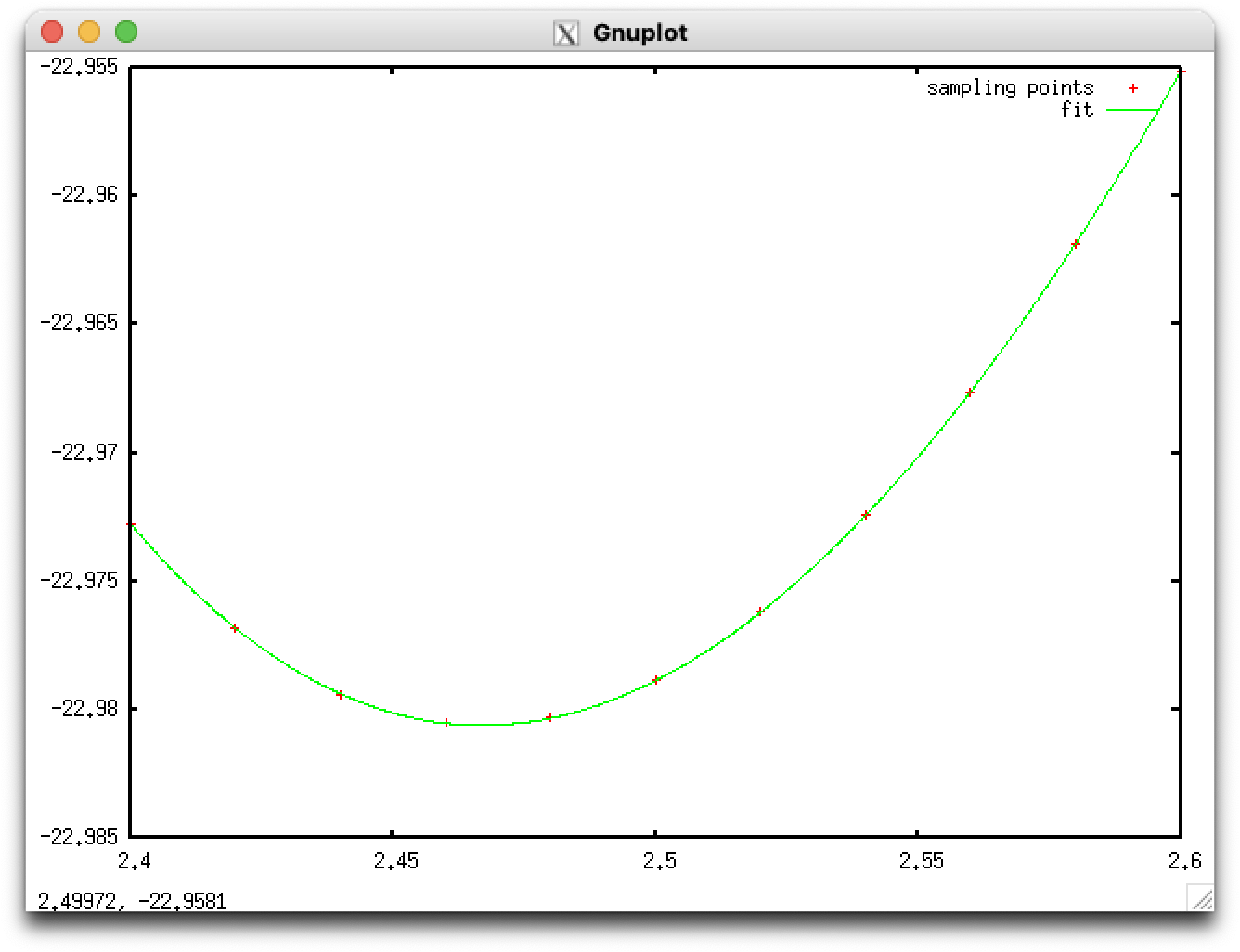
The equilibrium lattice constant can be obtained by fitting the total energy to, for instance, a polynomial. For example, the third-order polynomial. Result of fitting may look like:
The equilibrium lattice parameter thus obtained is 2.467 Angstrom.
Structural optimization with the variable cell relaxation †
Cell optimization can be also performed by using "vc-relax" with the following input file
&control
 calculation  = 'vc-relax'
 restart_mode = 'from_scratch',
 pseudo_dir   =  '/home/ikutaro/QE/pseudo',
 outdir       = './tmp'
 prefix       = 'gr'
 tstress      = .true.
 tprnfor      = .true.
/
&system
 ibrav       = 4
 A           = 2.46
 C           = 10.00
 nat         = 2
 ntyp        = 1
 ecutwfc     = 40.0
 ecutrho     = 400.0
 occupations = 'smearing'
 smearing    = 'mp'
 degauss     = 0.02
/
&electrons
 diagonalization = 'david'
 conv_thr        = 1.0e-12
 mixing_beta     = 0.5
/
&ions
/
&cell
 press          = 0.0d0
 press_conv_thr = 0.5d0
 cell_dofree    = 2Dxy
/
ATOMIC_SPECIES
 C  12.01070 c_pbe_v1.2.uspp.F.UPF
ATOMIC_POSITIONS (crystal)
  C 0.0000000000000000 0.0000000000000000 0.0000000000000000
  C 0.3333333333333333 0.6666666666666667 0.0000000000000000
K_POINTS (automatic)
 12 12 01 0 0 0
In this example, GBRV ultrasoft pseudopotential, cutoff energies of 40 and 400 Ry, and nonshifted 12 x 12 uniform k-point mesh is used. The vacuum of 10 Angstrom is inserted to separate periodic images. For the cell relaxation in two dimension, 'cell_dofree=2Dxy' is used.
SCF and band structure calculations †
Having relaxed the cell parameters, let us start the band structure calculation. In this tutorial, band structure calculations are performed by varying the k-point mesh in the SCF calculation to learn how the number of k-points or k-point density is crucial to determine the position of Fermi level and thereby the location of the Dirac point at the K point.
- SCF calculation
&control
 calculation  = 'scf'
 restart_mode = 'from_scratch',
 pseudo_dir   =  '/home/ikutaro/QE/pseudo',
 outdir       = './tmp'
 prefix       = 'gr'
 tstress      = .true.
 tprnfor      = .true.
/
&system
 ibrav       = 4
 A           = 2.46575870
 C           = 10.00
 nat         = 2
 ntyp        = 1
 ecutwfc     = 40.0
 ecutrho     = 400.0
 occupations = 'smearing'
 smearing    = 'mp'
 degauss     = 0.02
 nbnd        = 8
/
&electrons
 diagonalization = 'david'
 conv_thr        = 1.0e-12
 mixing_beta     = 0.5
/
&ions
/
&cell
 press          = 0.0d0
 press_conv_thr = 0.5d0
 cell_dofree    = 2Dxy
/
ATOMIC_SPECIES
 C  12.01070 c_pbe_v1.2.uspp.F.UPF
ATOMIC_POSITIONS (crystal)
  C 0.0000000000000000 0.0000000000000000 0.0000000000000000
  C 0.3333333333333333 0.6666666666666667 0.0000000000000000
K_POINTS (automatic)
 12 12 01 0 0 0
- Band structure
&control
 calculation  = 'bands'
 restart_mode = 'from_scratch',
 pseudo_dir   =  '/home/ikutaro/QE/pseudo',
 outdir       = './tmp'
 prefix       = 'gr'
 tstress      = .true.
 tprnfor      = .true.
/
&system
 ibrav       = 4
 A           = 2.46575870
 C           = 10.00
 nat         = 2
 ntyp        = 1
 ecutwfc     = 40.0
 ecutrho     = 400.0
 occupations = 'smearing'
 smearing    = 'mp'
 degauss     = 0.02
 nbnd        = 8
/
&electrons
 diagonalization = 'david'
 conv_thr        = 1.0e-12
 mixing_beta     = 0.5
/
&ions
/
&cell
 press          = 0.0d0
 press_conv_thr = 0.5d0
 cell_dofree    = 2Dxy
/
ATOMIC_SPECIES
 C  12.01070 c_pbe_v1.2.uspp.F.UPF
ATOMIC_POSITIONS (crystal)
  C 0.0000000000000000 0.0000000000000000 0.0000000000000000
  C 0.3333333333333333 0.6666666666666667 0.0000000000000000
K_POINTS (crystal_b)
4
  0.00000000  0.00000000  0.00000000 20.0
  0.66666667 -0.33333333  0.00000000 20.0
  0.50000000  0.00000000  0.00000000 20.0
  0.00000000  0.00000000  0.00000000  0.0
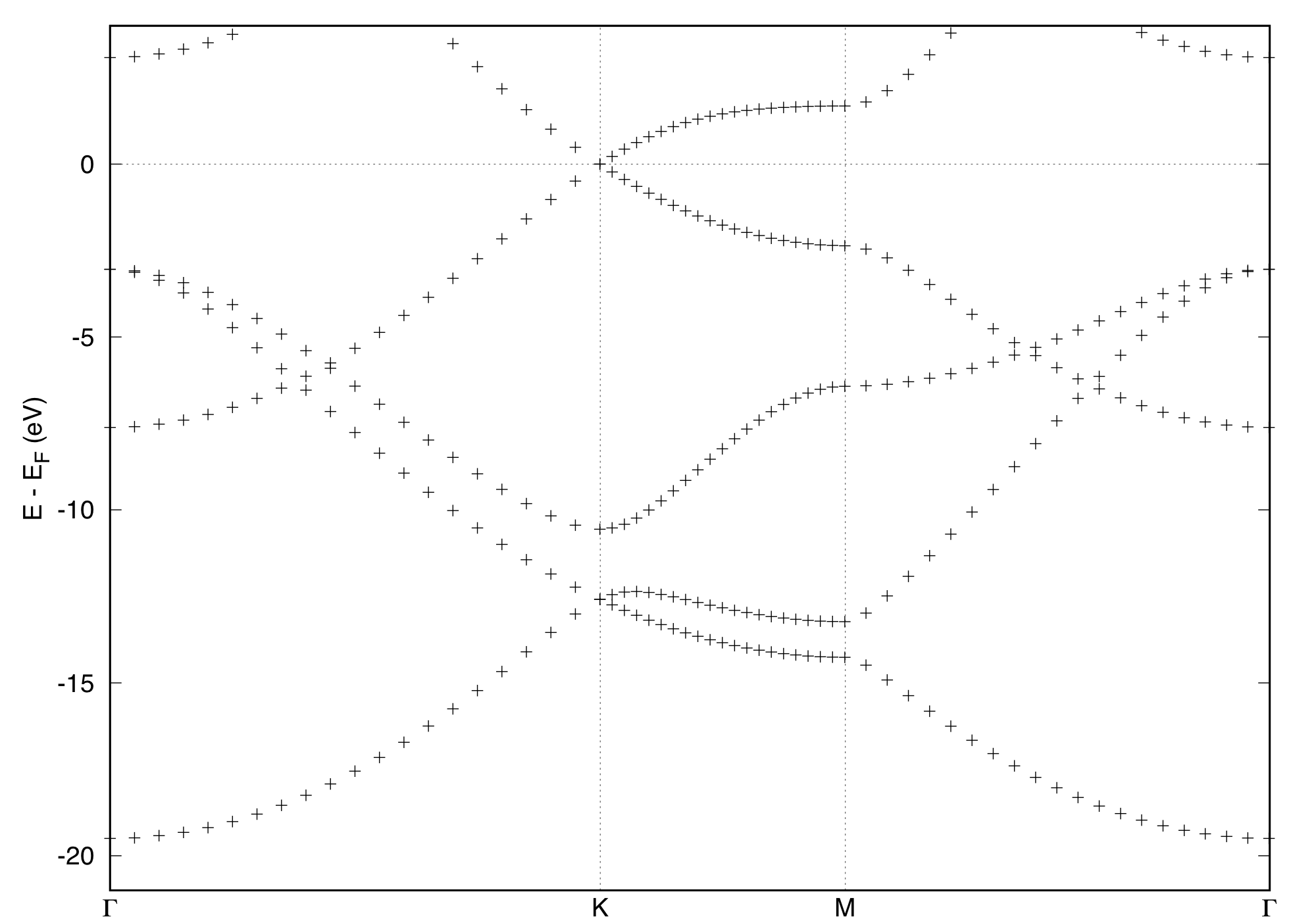
In this example, the energy band is draw along the Gamma-K-M-Gamma line. The symmetry points are given in the unit of basic reciprocal lattice vectors. Alternatively one can define high symmetry k-points by using strings as follows:K_POINTS (crystal_b) 4 gG 20.0 K 20.0 M 20.0 gG 0.0
In this, case ibrav should be specified properly in the &system.../ block. See Doc/brillouin_zones.pdf for the definition of the high-symmetry k-point labels (if brillouin_zone.pdf does not exist, type ``make`` in the Doc/ directory). - Post-processing
To plot the band structure with gnuplot or alike, "bands.x" is used. Here's an example of the input file (pp_bands.in):&bands outdir = './tmp' prefix = 'gr' filband = 'gr.bands' lsym = .true. /
Note that the same number of processors as the previous band structure calculation should be used. With this input, "gr.bands.gnu" and "gr.bands.rap" are generated. For use with gnuplot, "gr.bands.gnu" can be used. One can use the following script ("band_plot.sh") to generate the band plot with gnuplot#!/bin/sh ef=`grep Fermi gr_scf.out | awk '{print $5}'` gnuplot <<EOF ef=${ef} xmin=0.0 xmax=1.5784 ymin=-21.0 ymax=4.0 g1=0.0 k=0.6671 m=1.0007 g2=1.5784 offset=0.5 set arrow from k,ymin to k,ymax nohead lt 0 set arrow from m,ymin to m,ymax nohead lt 0 unset xtics set ylabel 'E - E_F (eV)' set label '{/Symbol G}' at g1,ymin-offset center set label 'K' at k,ymin-offset center set label 'M' at m,ymin-offset center set label '{/Symbol G}' at g2,ymin-offset center set xrange [xmin:xmax] set yrange [ymin:ymax] set xzeroaxis lt 0 plot 'gr.bands.gnu' using (\$1):(\$2-ef) pause -1 EOFand type$ sh band_plot.sh
Here the output file for the corresponding SCF calculation is assumed to be "gr.scf.out." If you want to save the band structure change the terminal in gnuplot as#!/bin/sh ef=`grep Fermi gr_scf.out | awk '{print $5}'` gnuplot <<EOF ef=${ef} xmin=0.0 xmax=1.5784 ymin=-21.0 ymax=4.0 g1=0.0 k=0.6671 m=1.0007 g2=1.5784 offset=0.5 set arrow from k,ymin to k,ymax nohead lt 0 set arrow from m,ymin to m,ymax nohead lt 0 unset xtics set ylabel 'E - E_F (eV)' set label '{/Symbol G}' at g1,ymin-offset center set label 'K' at k,ymin-offset center set label 'M' at m,ymin-offset center set label '{/Symbol G}' at g2,ymin-offset center set xrange [xmin:xmax] set yrange [ymin:ymax] set xzeroaxis lt 0 set terminal postscript eps set output 'gr.bands.eps' plot 'gr.bands.gnu' using (\$1):(\$2-ef) pause -1 EOFThe figure for the band structure is written to 'gr.bands.eps.'
Exercise †
- In this tutorial, relatively large cutoff energies (ecutwfc = 40 Ry and ecutrho = 400 Ry) were used and the optimized lattice parameter is reasonablly accurate. However, the convergence of lattice parameter with respect to the cutoff should be always checked. Increase and decrease ecutwfc and ecutrho and choose the optimum cutoffs. Remember ecutrho > ecutwfc * 4 when the ultrasoft pseudopotentials are used.
- The position of the Dirac cone at the K-point should be located at the Fermi level. However, the position of the Fermi level is very sensitive to the number of k-point. Examine how many k-points (how dense the k-point mesh) starting from, for e.g., 6x6x1, 8x8x1, ... 12x12x1.
![[PukiWiki] [PukiWiki]](image/logo_state-senri3_80x80.png)

