
To enter CMD2 server, you use ssh command with your own RSA private key:
$ ssh -i .ssh/id_rsa -Y your_id@cmd2.phys.sci.osaka-u.ac.jp
Enter passphrase for key '.ssh/id_rsa': ********
A compressed file of the State code is obtained from the following directory.
So let's copy (cp) and decompress (tar xzvf) the .tgz file:
$ cp /home/CMD/teac17/STATE/archives/state-cmd35.tgz .
$ tar xzvf state-cmd35.tgz
$ ls
STATE  state-cmd35.tgz
If you change directory (cd) to STATE,
you can find the following file and directories:
$ cd STATE
$ ls
README  arch  build  example  gncpp  src  util
| Directory | Description |
|---|---|
example |
Examples used in this tutorial |
gncpp |
Pseudopotential files |
src |
Source codes of State |
util |
Utility scripts |
The examples used in this tutorial are contained in example directory:
$ cd example
$ ls
Al  C2H4  C2H4_FTMD  CLEANUP  CO  ClonAl100  Mg  Na  Ni  README  Si
Directory Na initilly contains the following directory and files:
$ cd Na
$ ls
References  nfinp_1  qsub.sh
| File or directory | Description |
|---|---|
References |
Directory containing output files as a reference |
nfinp_1 |
Input file |
qsub.sh |
Job script file |
The input file nfinp_1 reads:
$ cat nfinp_1
     0     0     0     0     0     0
  4.00 10.00     1     1     1       : GMAX GMAXP NTYP NATM NATM2
   229     1                         : NUM_SPACE_GROUP TYPE_BRAVAIS_LATTICE
  7.90  7.90  7.90 90.00 90.00 90.00 : A B C ALPHA BETA GAMMA
    12    12    12     1     1     1
     0     0
  0.00  0.00  0.00     1     0     1
    11  0.50 22.99     6     1   0.2 : IATOMN ALFA AMION ILOC IVAN
     0     0     0     0     0     0
     0     1
    20    20     0    84200.00     0
     6     1
     0    20  0.60
  0.20  0.30  0.20  0.20  0.20
300.00     4     1    0.50D-09       : DTIO IMDALG IEXPL EDELTA
-10.0002  0.50D+03     0
ggapbe     1
  2.00
   101
     4     4     4
     4     4     4
     6
     1
     0
     2
     0
     0
     0  0.00
| Parameter | Value | Description |
|---|---|---|
NTYP |
1 |
Number of atomic species |
NATM |
1 |
Number of atoms |
NATM2 |
1 |
Number of atoms (= NATM) |
NUM SPACE GROUP |
229 |
Space group number (refer to e.g. this page) |
BRAVAIS LATTICE |
1 |
Body-centered cubic |
A |
7.90 |
Length of lattice vector $\boldsymbol{A}$ in Bohr |
B |
7.90 |
Length of lattice vector $\boldsymbol{B}$ in Bohr |
C |
7.90 |
Length of lattice vector $\boldsymbol{C}$ in Bohr |
ALPHA |
90.0 |
Angle between $\boldsymbol{B}$ and $\boldsymbol{C}$ in degree |
BETA |
90.0 |
Angle between $\boldsymbol{C}$ and $\boldsymbol{A}$ in degree |
GAMMA |
90.0 |
Angle between $\boldsymbol{A}$ and $\boldsymbol{B}$ in degree |
IATOMN |
11 |
Atomic number |
EDELTA |
0.50D-09 |
Energy threshold for convergence in Hartree |
The job script is submitted using qsub command:
$ qsub qsub.csh
Your job 85 ("Na") has been submitted
If the calculation is finished successfully, some files are created in the current directory:
$ ls
Na.e85  Na.pe85  References  dos.data  nfinp_1  nfstop.data     qsub.sh
Na.o85  Na.po85  STATE       fort.37   nfout_1  potential.data  zaj.data
| File | Description |
|---|---|
dos.data |
Density of states (DOS) |
nfstop.data |
The job is stopped if 1 is written (i.e. cat 1 > nfstop.data) |
nfout_1 |
Output file |
potential.data |
Effective potential or charge density |
zaj.data |
Wave functions |
The convergence of total energy can be seen by extracting lines including "ETOT:" from nfout_1:
$ grep ETOT: nfout_1
ETOT:   1     -0.70836409  0.7084E+00  0.1446E-03
ETOT:   2     -0.88173590  0.1734E+00  0.4949E-03
ETOT:   3     -0.89514126  0.1341E-01  0.2566E-03
ETOT:   4     -0.89514200  0.7358E-06  0.4164E-04
ETOT:   5     -0.89514201  0.1375E-07  0.7103E-05
ETOT:   6     -0.89514201  0.1805E-08  0.5763E-06
ETOT:   7     -0.89514201  0.1652E-10  0.6293E-07
ETOT:   8     -0.89514201  0.2537E-11  0.4071E-07
ETOT:   9     -0.89514201  0.1709E-11  0.5460E-08
The total energy has converged to $-0.89514201$ Hartree after nine iterations,
when energy fluctuation $0.1709\times10^{-11}$ Hartree falls below EDELTA.
To take a glance at dos.data, it is convenient to use command head or tail,
which shows only the first or last ten lines:
$ head dos.data
    -13.5948134416      0.0000000000      0.0000000000
    -13.5839288832      0.0000000000      0.0000000000
    -13.5730443248      0.0000000000      0.0000000000
    -13.5621597664      0.0000000000      0.0000000000
    -13.5512752080      0.0000000000      0.0000000000
    -13.5403906496      0.0000000000      0.0000000000
    -13.5295060912      0.0000000000      0.0000000000
    -13.5186215328      0.0000000000      0.0000000000
    -13.5077369744      0.0000000000      0.0000000000
    -13.4968524160      0.0000000000      0.0000000000
$ tail dos.data
      8.0654577744      0.4295924878      0.4718856059
      8.0763423328      0.4300690051      0.4746348279
      8.0872268912      0.4305320052      0.4772607389
      8.0981114496      0.4301968559      0.4797567493
      8.1089960080      0.4295186395      0.4821169471
      8.1198805664      0.4455473921      0.4843361241
      8.1307651248      0.4395926656      0.4864097972
      8.1416496832      0.4345516132      0.4883342254
      8.1525342416      0.4342525693      0.4901064214
      8.1634188000      0.4317972913      0.4917241594
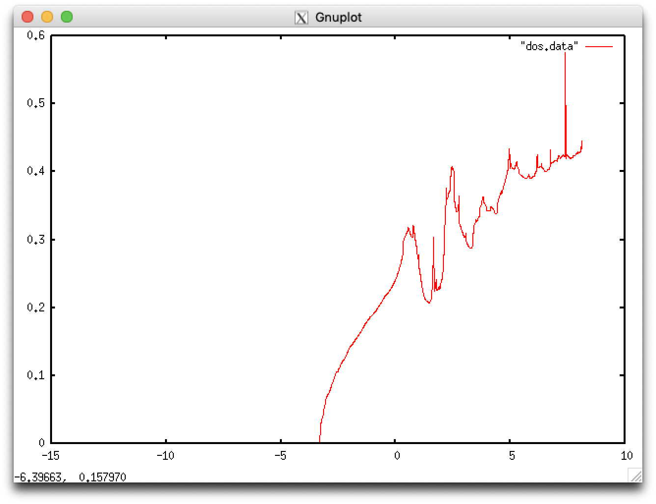
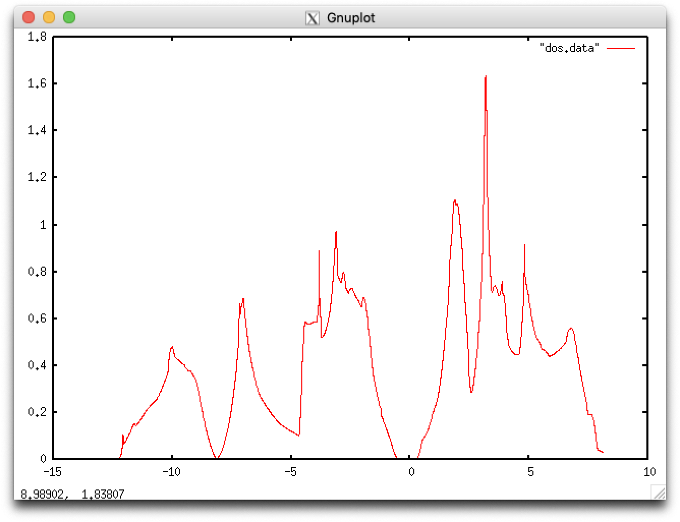
The first column corresponds to energy in eV,
while the second and third to raw and smeared data of DOS,
respectively, in eV$^{-1}$.
dos.data can be visualized by using e.g. gnuplot:
$ gnuplot

    G N U P L O T
    Version 4.6 patchlevel 2    last modified 2013-03-14
    Build System: Linux x86_64

    Copyright (C) 1986-1993, 1998, 2004, 2007-2013
    Thomas Williams, Colin Kelley and many others

    gnuplot home:     http://www.gnuplot.info
    faq, bugs, etc:   type "help FAQ"
    immediate help:   type "help"  (plot window: hit 'h')

Terminal type set to 'x11'
gnuplot> plot "dos.data" with lines

$ cd ../Mg
$ cat nfinp_1
     0     0     0     0     0     0
  4.00  8.00     1     2     2       : GMAX GMAXP NTYP NATM NATM2
   194     0                         : NUM_SPACE_GROUP TYPE_BRAVAIS_LATTICE
  6.10  6.10  9.60  90.0  90.0 120.0 : A B C ALPHA BELTA GAMMA
    12    12     8     1     1     1
     0     0                         : NCORD  NINV :IWEI IMDTYP ITYP
     0.3333333333333  0.666666666667  0.2500000000  1  0  1
    -0.3333333333333 -0.666666666667 -0.2500000000  1  0  1
    12  0.20 24.31     6     1   0.0 : IATOMN ALFA AMION ILOC IVAN
     0     0     0     0     0
     0     1
    50    50     0    36000.00     0
     6     1
     0    30   0.6
   0.2   0.3  0.20  0.20  0.20
 30.00     1     1     0.10D-9
 -10.0020  0.50D+05        0
GGAPBE     1
  1.00     3
   101
     2     2     2
     2     2     2
     8
     1
     0
     2
     0
     0
     0   0.0
| Parameter | Value | Description |
|---|---|---|
NATM |
2 |
Two Mg atoms in a primirive cell |
NUM SPACE GROUP |
194 |
Space group number of $P6_3/mmc$ |
BRAVAIS LATTICE |
0 |
Simple cubic |
NCORD |
0 |
Coodinates in units of lattice vectors |
IATOMN |
12 |
Atomic number of Mg |
$ qsub qsub.sh
Your job 87 ("Mg") has been submitted
$ grep ETOT: nfout_1
ETOT:   1    -11.69218799  0.1169E+02  0.4000E-02
ETOT:   2    -12.57326963  0.8811E+00  0.1936E-02
ETOT:   3    -12.58097106  0.7701E-02  0.9814E-03
ETOT:   4    -12.58105558  0.8451E-04  0.6903E-04
ETOT:   5    -12.58105821  0.2634E-05  0.1438E-04
ETOT:   6    -12.58105817  0.4680E-07  0.1344E-05
ETOT:   7    -12.58105814  0.2291E-07  0.4425E-06
ETOT:   8    -12.58105814  0.2388E-08  0.3259E-07
ETOT:   9    -12.58105814  0.1666E-09  0.5973E-08
ETOT:  10    -12.58105814  0.1011E-09  0.1165E-08
ETOT:  11    -12.58105814  0.1202E-10  0.2957E-09
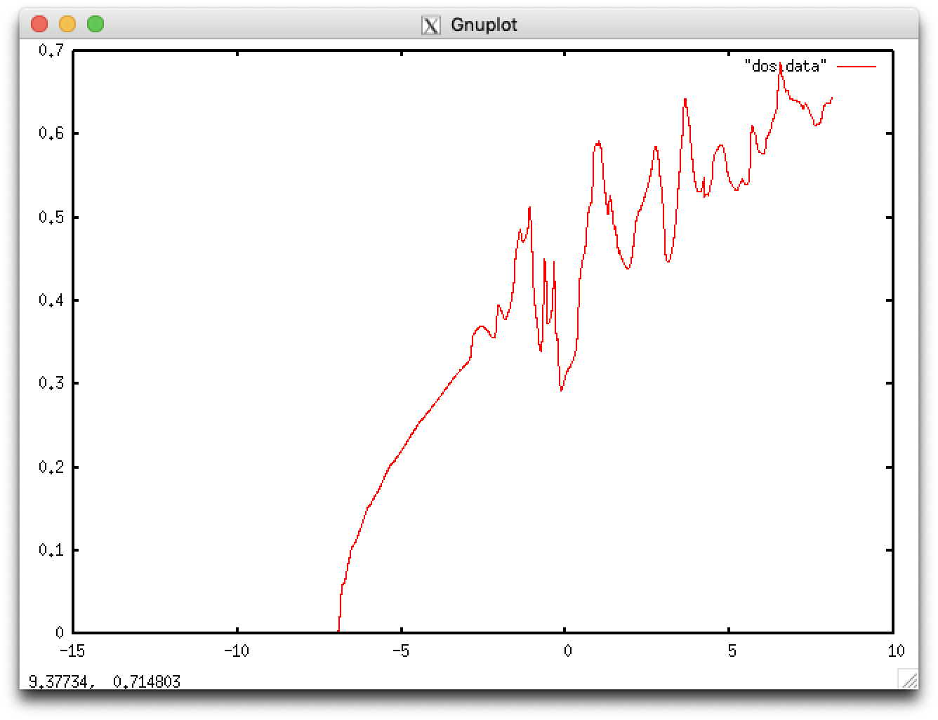
$ gnuplot
gnuplot> plot "dos.data" with lines
We here learn how to optimize the lattice constants of solids.

$ cd ../Al
$ cat nfinp_1
     0     0     0     0     0     0
  4.00  8.00     1     1     1       : GMAX GMAXP NTYP NATM NATM2
   221     2                         : NUM_SPACE_GROUP TYPE_BRAVAIS_LATTICE
  7.60  7.60  7.60 90.00 90.00 90.00 : A B C ALPHA BETA GAMMA
    12    12    12     1     1     1
     0     0
  0.00  0.00  0.00     1     0     1
    13  0.50 26.98     6     1  0.20 : IATOMN ALFA AMION ILOC IVAN
     0     0     0     0     0
     0     1
    30    30     0     84200.00    0
     6     1
     0    20  0.60
  0.20  0.30  0.20  0.20  0.20
300.00     4     1    0.50D-09
-0.0020   0.50D+03     0
ggapbe     1
  2.00
   101
     4     4     4
     4     4     4
     6
     1
     0
     2
     0
     0
     0  0.00
| Parameter | Value | Description |
|---|---|---|
NATM |
1 |
One Al atoms in a primirive unit cell |
NUM SPACE GROUP |
221 (225) |
Space group number of $Pm\overline{3}m$ ($Fm\overline{3}m$) |
BRAVAIS LATTICE |
2 |
Face-centered cubic |
IATOMN |
13 |
Atomic number of Al |
We vary lattice constants A, B and C from 7.5 Bohr to 7.9 Bohr and compare calculated energies to see at which value the system is most stabilized.
The input files for repective cases are:
$ ls nfinp_*.*
nfinp_7.5  nfinp_7.6  nfinp_7.7  nfinp_7.8  nfinp_7.9
The lattice constants for these input files can be seen by extracting (grep) lines including a,b,c:
$ grep "a,b,c" nfinp_*.*
nfinp_7.5:7.5 7.5 7.5 90.000 90.000 90.000 : a,b,c,alpha,beta,gamma
nfinp_7.6:7.6 7.6 7.6 90.000 90.000 90.000 : a,b,c,alpha,beta,gamma
nfinp_7.7: 7.700000 7.700000 7.700000 90.000 90.000 90.000 : a,b,c,alpha,beta,gamma
nfinp_7.8:7.8 7.8 7.8 90.000 90.000 90.000 : a,b,c,alpha,beta,gamma
nfinp_7.9:7.9 7.9 7.9 90.000 90.000 90.000 : a,b,c,alpha,beta,gamma
The last block in qsub.sh
for a in 7.5 7.6 7.7 7.8 7.9
do
  mpirun -np $NSLOTS ./STATE < nfinp_${a} > nfout_${a}
done
means that STATE reads these input files sequentially.
$ qsub qsub.sh
Your job 202 ("Al") has been submitted
The output files for respective lattice constants are
$ ls nfout_7.*
nfout_7.5  nfout_7.6  nfout_7.7  nfout_7.8  nfout_7.9
For $a=7.5$ Bohr, the total energy converges to $-2.07149828$ Hartree:
grep ETOT: nfout_7.5
ETOT:   1     -1.61454558  0.1615E+01  0.2131E-02
ETOT:   2     -2.06781187  0.4533E+00  0.3173E-02
ETOT:   3     -2.07148674  0.3675E-02  0.1291E-02
ETOT:   4     -2.07149811  0.1138E-04  0.2187E-03
ETOT:   5     -2.07149826  0.1450E-06  0.4815E-04
ETOT:   6     -2.07149828  0.2419E-07  0.1976E-05
ETOT:   7     -2.07149828  0.3317E-09  0.4737E-06
ETOT:   8     -2.07149828  0.8983E-10  0.3199E-07
ETOT:   9     -2.07149828  0.5185E-10  0.5603E-08
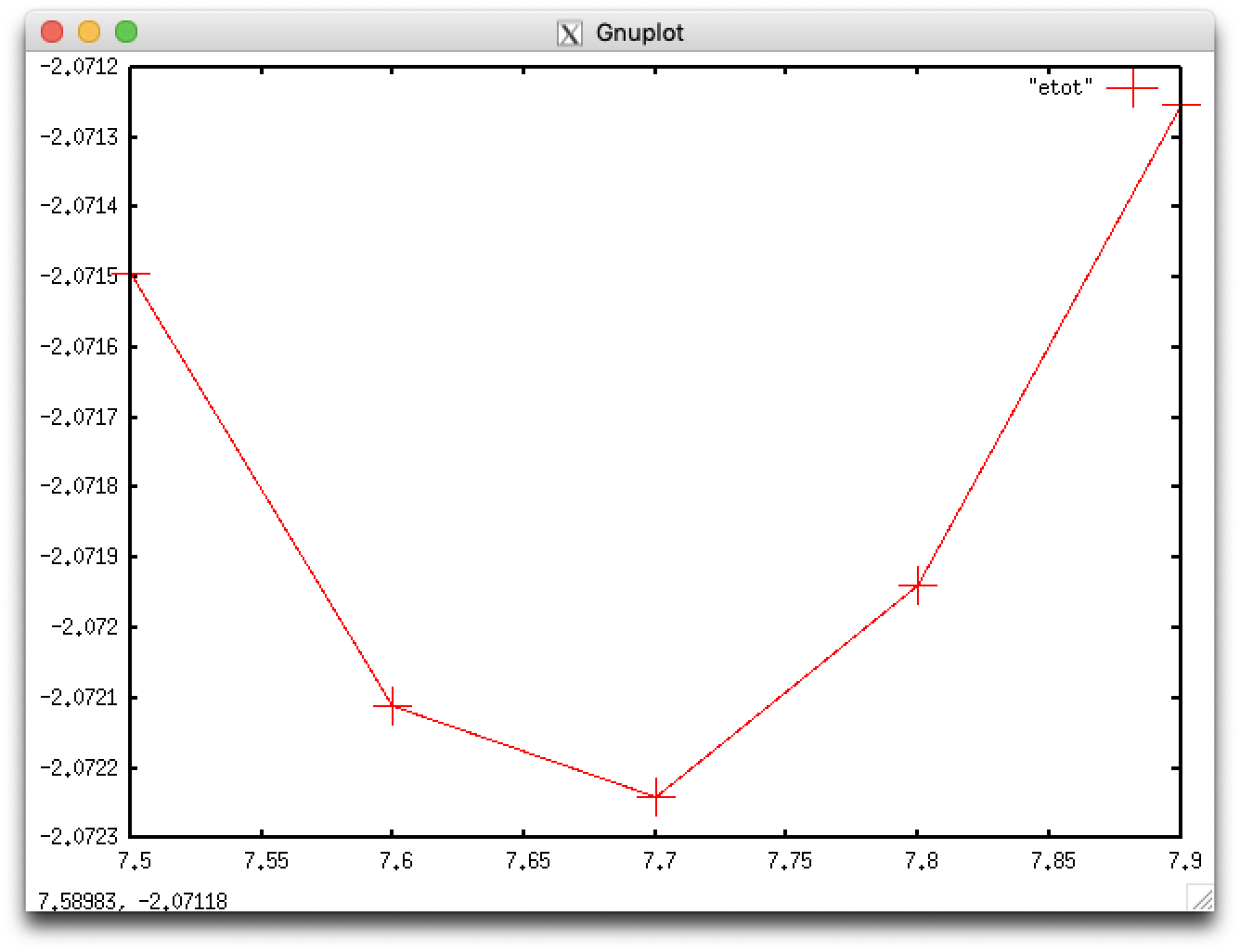
The total energies for respective lattice constants can be obtained by using script getetot.sh contained in the current directory:
$ ./getetot.sh
7.5 -2.07149508
7.6 -2.07210987
7.7 -2.07223992
7.8 -2.07193773
7.9 -2.07125357
This indicates that the lattice constans are optimized at $a\lesssim 7.7$ Bohr. Fully optimized lattice constans are obtained from least-squares fittng:
$ ./getetot.sh > etot
$ gnuplot
gnuplot> plot "etot" with linespoints pointsize 5
We fit the five data points with a parabolic curve \[ f(x)=ax^2+bx+c \]
gnuplot> f(x)=a*x**2+b*x+c
gnuplot> fit f(x) "etot" via a,b,c
.
.
.
Final set of parameters            Asymptotic Standard Error
=======================            ==========================

a               = 0.0216439        +/- 0.0006142    (2.838%)
b               = -0.33266         +/- 0.009459     (2.843%)
c               = -0.794021        +/- 0.03641      (4.585%)


correlation matrix of the fit parameters:

               a      b      c
a               1.000
b              -1.000  1.000
c               1.000 -1.000  1.000
gnuplot> plot "etot" pointsize 5, f(x)
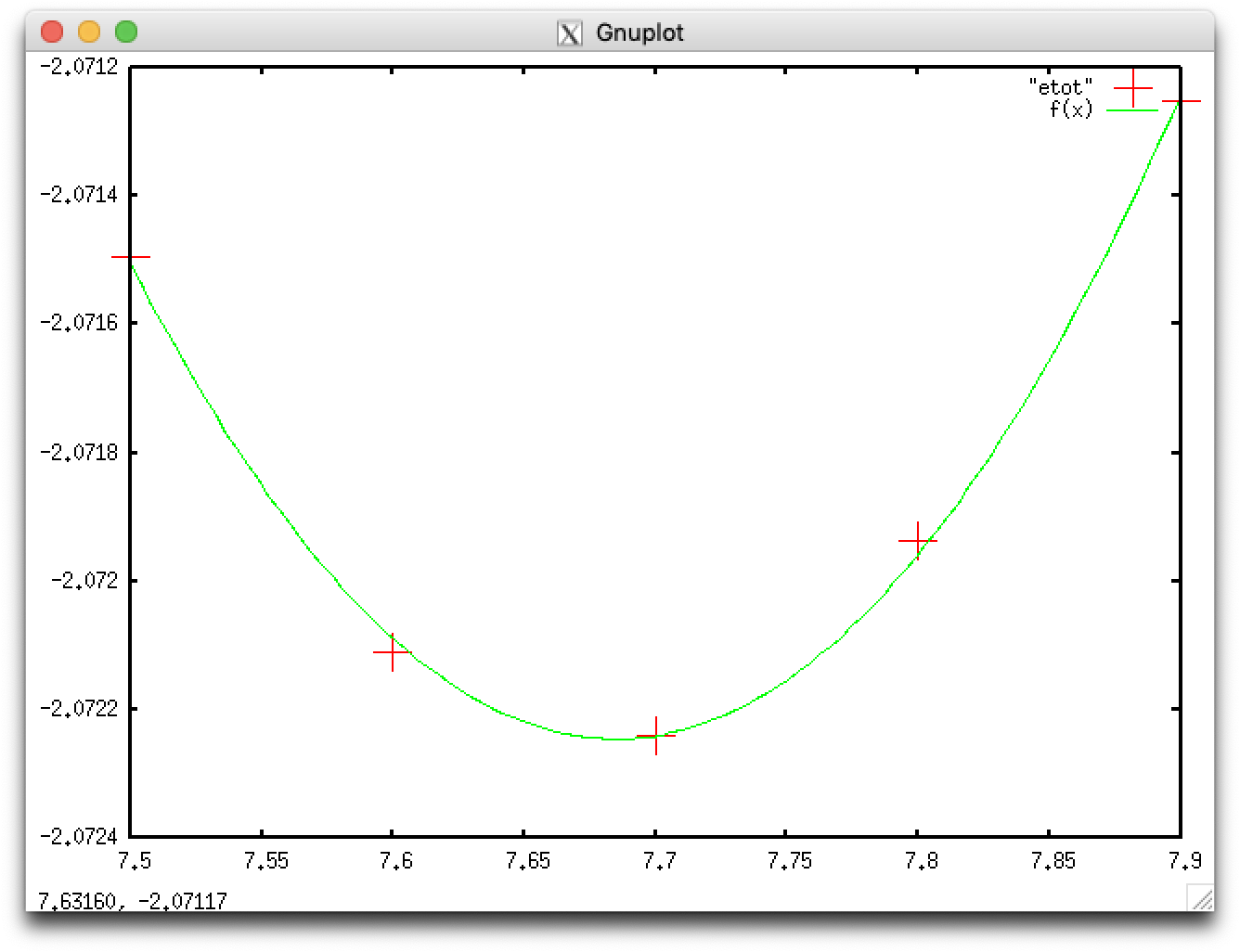
The optimal lattice constants are obtained by calculating $-\frac{b}{2a}$
$ echo "0.33266/2/0.0216439" | bc -l
7.68484422862792749920
We here consider a semiconductor with a band gap.

$ cd ../Si
$ cat nfinp_1
     0     0     0     0     0     0
  4.00  8.00     1     2     2       : GMAX, GMAXP, NTYP, NATM, NATM2
   227     2                         : NUM_SPACE_GROUP TYPE_BRAVAIS_LATTICE
 10.30 10.30 10.30 90.00 90.00 90.00
    08    08    08     1     1     1
     0     0
0.00d0      0.00d0      0.00d0    1    1    1
0.25d0      0.25d0      0.25d0    1    1    1
    14  0.50 28.09     6     1   0.2 : TYPE 1IATOMN,ALFA,AMION,ILOC,IVAN
     0     0     0     0     0
     0     1
    20    20     0    84200.00     0
     6     1
     0    20  0.60
     0.20  0.30  0.20  0.20  0.20
   300.00  4     1    0.50D-09
0.0002    0.50D+03     0
ggapbe     1
  2.00
   102
     4     4     4
     4     4     4
     8
     1
     0
     2
     0
     2
     1
     2
-15.00  5.00  0.20   501
 2.400  0.20
        0.20    14
     0  0.00
| Parameter | Value | Description |
|---|---|---|
NATM |
2 |
Two Si atoms in a primitive cell |
NUM SPACE GROUP |
227 |
Space group number of $Fd\overline{3}m$ |
TYPE BRAVAIS LATTICE |
2 |
Face-centered cubic |
IATOMN |
14 |
Atomic number of Si |
$ qsub qsub.sh
Your job 823 ("Si") has been submitted
$ grep ETOT: nfout_1
ETOT:   1     -6.05513096  0.6055E+01  0.3203E-02
ETOT:   2     -7.84016187  0.1785E+01  0.5187E-02
ETOT:   3     -7.87270490  0.3254E-01  0.2825E-02
ETOT:   4     -7.87351715  0.8123E-03  0.6089E-03
ETOT:   5     -7.87355245  0.3530E-04  0.1887E-03
ETOT:   6     -7.87355822  0.5769E-05  0.2560E-04
ETOT:   7     -7.87355833  0.1069E-06  0.1066E-04
ETOT:   8     -7.87355833  0.4548E-08  0.1730E-05
ETOT:   9     -7.87355833  0.1916E-09  0.4194E-06
ETOT:  10     -7.87355833  0.2984E-10  0.1669E-07
ETOT:  11     -7.87355833  0.1943E-11  0.9524E-08
$ gnuplot
gnuplot> plot "dos.data" with lines
The cauclated energy gap of 0.7 eV is smaller than experimental results of 1.1 eV. Such underestimation of energy gaps is a well-known behavior of DFT results.
We here consider a ferromagnet with spin polarization.
$ cd ../Ni
$ cat nfinp_1
     0     0     0     0     0     0
  5.00 15.00     1     1     1
   221     2
  6.70  6.70  6.70 90.00 90.00 90.00
    12    12    12     1     1     1
     0     0
  0.00  0.00  0.00     1     0     1
    28  0.50 58.69     6     1   0.1 : IATOMN,ALFA,AMION,ILOC,IVAN,ZETA1
     0     0     0     0     0
     0     1
    30    30     0    84200.00     0
     6     1
     0    20  0.30
  0.20  0.30  0.20  0.20  0.20
300.00     4     1    0.50D-09
-0.002    0.50D+03     0
ggapbe     2                         : XCTYPE,KSPIN
  2.00
   101
     4     4     4
     4     4     4
    10
     1
     0
     2
     0
     1
     1
-15.00  5.00  0.20   501
     2.40000    0.200000
     0.20000    14
     0  0.00
| Parameter | Value | Description |
|---|---|---|
ZETA1 |
0.1 |
Initial value of relative spin polarization |
KSPIN |
2 |
Charge densities for up and down spins are treated separately |
Definition of relative spin polarization \[ \zeta=\frac{N_\uparrow-N_\downarrow}{N_\uparrow+N_\downarrow} \]
$ qsub qsub.sh
Your job 1071 ("Ni") has been submitted
$ grep ETOT: nfout_1
ETOT:   1    -48.03422182  0.4803E+02  0.1740E-01
ETOT:   2    -48.09018411  0.5596E-01  0.2913E-01
ETOT:   3    -48.35445050  0.2643E+00  0.4213E-02
ETOT:   4    -48.35581458  0.1364E-02  0.3191E-02
ETOT:   5    -48.35596078  0.1462E-03  0.2878E-02
ETOT:   6    -48.35603500  0.7422E-04  0.3500E-02
ETOT:   7    -48.35608363  0.4863E-04  0.2013E-02
ETOT:   8    -48.35608557  0.1938E-05  0.1434E-02
ETOT:   9    -48.35609022  0.4651E-05  0.3847E-03
ETOT:  10    -48.35609188  0.1668E-05  0.1860E-03
ETOT:  11    -48.35609244  0.5604E-06  0.6846E-04
ETOT:  12    -48.35609276  0.3143E-06  0.4412E-05
ETOT:  13    -48.35609276  0.2773E-08  0.4316E-05
ETOT:  14    -48.35609277  0.1732E-07  0.7494E-06
ETOT:  15    -48.35609278  0.2083E-08  0.2593E-06
ETOT:  16    -48.35609278  0.1319E-08  0.5970E-07
ETOT:  17    -48.35609278  0.1041E-09  0.3455E-07
ETOT:  18    -48.35609278  0.6774E-10  0.2829E-07
ETOT:  19    -48.35609278  0.1236E-09  0.9241E-08
Spin polarization can be confirmed by extracting lines including "Charge Density =" from nfout_1:
$ grep "Charge Density = " nfout_1 | sed -e "s/^.*=//"
   5.5000000000   4.5000000000  10.0000000000
   5.5000000000   4.5000000000  10.0000000000
   5.0000004105   5.0000004281   9.9999991614
   5.2578321672   4.7421678328  10.0000000000
   5.3398749142   4.6601246078  10.0000004781
   5.2975685186   4.7024314814  10.0000000000
   5.2859332950   4.7140669339   9.9999997711
   5.2922061685   4.7077938315  10.0000000000
   5.3141836552   4.6858164843   9.9999998605
   5.3013843445   4.6986156555  10.0000000000
   5.3345599671   4.6654401481   9.9999998848
   5.4563714243   4.5436285757  10.0000000000
   5.3608062331   4.6391938548   9.9999999121
   5.4119364707   4.5880635293  10.0000000000
   5.3595085386   4.6404915449   9.9999999164
   5.3969604451   4.6030395549  10.0000000000
   5.3598549611   4.6401451225   9.9999999164
   5.3636681705   4.6363318295  10.0000000000
   5.3540235787   4.6459765078   9.9999999135
   5.3562830503   4.6437169497  10.0000000000
   5.3517383485   4.6482617376   9.9999999139
   5.3518121053   4.6481878947  10.0000000000
   5.3501642704   4.6498358163   9.9999999133
   5.3494996637   4.6505003363  10.0000000000
   5.3494117687   4.6505883184   9.9999999129
   5.3495529688   4.6504470312  10.0000000000
   5.3494412221   4.6505588648   9.9999999131
   5.3494258883   4.6505741117  10.0000000000
   5.3494045041   4.6505955829   9.9999999130
   5.3494083435   4.6505916565  10.0000000000
   5.3494011874   4.6505988996   9.9999999130
   5.3493965623   4.6506034377  10.0000000000
   5.3493981629   4.6506019240   9.9999999131
   5.3493972564   4.6506027436  10.0000000000
   5.3493983908   4.6506016962   9.9999999130
   5.3493977310   4.6506022690  10.0000000000
   5.3493985687   4.6506015183   9.9999999130
   5.3493985970   4.6506014030  10.0000000000
   5.3493988925   4.6506011945   9.9999999130
The first and second columns correspond to charges with up and down spins, respectively, while the third to the total charge. The initial and final values of relative spin polarization are \[ \zeta_{\rm ini}=\frac{5.50-4.50}{10.00}=0.10, \] \[ \zeta_{\rm fin}=\frac{5.34-4.65}{10.00}=0.07. \]
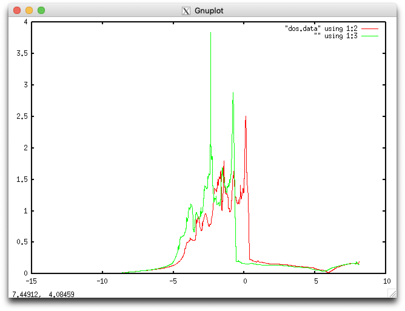
Unlike spin non-polarized calculations, dos.data consists of five columns:
$ head dos.data | tr -s " "
 -13.5948134416 0.0000000000 0.0000000000 0.0000000000 0.0000000000
 -13.5839288832 0.0000000000 0.0000000000 0.0000000000 0.0000000000
 -13.5730443248 0.0000000000 0.0000000000 0.0000000000 0.0000000000
 -13.5621597664 0.0000000000 0.0000000000 0.0000000000 0.0000000000
 -13.5512752080 0.0000000000 0.0000000000 0.0000000000 0.0000000000
 -13.5403906496 0.0000000000 0.0000000000 0.0000000000 0.0000000000
 -13.5295060912 0.0000000000 0.0000000000 0.0000000000 0.0000000000
 -13.5186215328 0.0000000000 0.0000000000 0.0000000000 0.0000000000
 -13.5077369744 0.0000000000 0.0000000000 0.0000000000 0.0000000000
 -13.4968524160 0.0000000000 0.0000000000 0.0000000000 0.0000000000
The second and third columns correspond to raw data for up and down spins, respectively, while the fourth and fifth to smeared data for up and down spins, respectively. Spin polarization can also be confirmed by plotting the DOS data for up and down spins:
$ gnuplot
gnuplot> plot "dos.data" using 1:2 with lines,"" using 1:3 with lines
We here consider a diatomic molecule in a vacuum.
Directory CO contains three input files corresponding to different diagonalization scheme:
$ cd ../CO
$ ls nfinp_*
nfinp_dav  nfinp_rmm1  nfinp_rmm2
The last block in qsub.sh
for j in dav rmm1 rmm2
do
  mpirun -np $NSLOTS ./STATE < nfinp_${j} > nfout_${j}
done
means that STATE reads these input files sequentially.
Among them, nfinp_dav reads:
$ cat nfinp_dav
     0     0     0     0     0     0
  5.50 20.00     2     2     2       : GMAX GMAXP NTYP NATM NATM2
     1     0                         : NUM_SPACE_GROUP TYPE_BRAVAIS_LATTICE
  6.00  4.00  4.00 90.00 90.00 90.00
     1     1     1     1     1     1
     1     0                         : NCORD, NINV
  0.00  0.00  0.00     1     1     1 : CPS(1,1:3) IWEI IMDTYP ITYP
  2.20  0.00  0.00     1     1     2 : CPS(2,1:3) IWEI IMDTYP ITYP
     6  0.15 12.01     3     1  0.d0 : IATOMN ALFA AMION ILOC IVAN
     8  0.15 16.00     3     1  0.d0 : IATOMN ALFA AMION ILOC IVAN
     0     0     0     0     0       : ICOND INIPOS INIVEL ININOS INIACC
     0     1
   200   200     0    57200.00     0
     3     1
     0     8   0.8
  0.60  0.50  0.60  0.70  1.00
 30.00     2     1    0.10D-08
 0.001    0.10D+02     0
ggapbe     1
  1.00
   102
     0     0     0
     0     0     0
     8
     1                               : NEXTST
     0
     2                               : IMSD
     0
     0
     0   0.0
| Parameter | Value | Description |
|---|---|---|
NTYP |
2 |
Two atomic species C and O |
NATM |
2 |
One C atom and one O atom in a primitive cell |
NUM SPACE GROUP |
1 |
Space group number of $P_1$ |
TYPE BRAVAIS LATTICE |
0 |
Simple cubic |
NCORD |
1 |
Coordinates in units of Bohr |
ITYP |
1 or 2 |
Index of atomic species in the position |
The difference among the input files can be seen by using command diff:
$ diff nfinp_dav nfinp_rmm1
11c11
<      0     0     0     0     0       : ICOND INIPOS INIVEL ININOS INIACC
---
>      1     0     0     0     0       : ICOND INIPOS INIVEL ININOS INIACC
25c25
<      1                               : NEXTST
---
>      0                               : NEXTST
27c27
<      2                               : IMSD
---
>      1                               : IMSD
$ diff nfinp_rmm1 nfinp_rmm2
27c27
<      1                               : IMSD
---
>      2                               : IMSD
| Parameter | Value | Description |
|---|---|---|
ICOND |
0 |
Start calculation from scratch with randomly generated wave functions |
1 |
Restart calculation using old wave functinos and charge density | |
NEXTST |
0 |
Non-local pseudopotentials in the real space |
1 |
Non-local pseudopotentials in the reciprocal space | |
IMSD |
1 |
Diagonalization by means of the RMM-DIIS method (faster than the Davidson method but applicable only near convergence) |
2 |
Diagonalization by means of the Davidson method |
$ qsub qsub.sh
Your job 1265 ("CO") has been submitted
$ grep ETOT: nfout_dav
ETOT:   1    -16.71058056  0.1671E+02  0.8965E-01
ETOT:   2    -20.04069483  0.3330E+01  0.6387E-01
ETOT:   3    -21.45761599  0.1417E+01  0.6830E-01
ETOT:   4    -22.15338988  0.6958E+00  0.2822E-01
ETOT:   5    -22.21588778  0.6250E-01  0.7654E-02
ETOT:   6    -22.21907373  0.3186E-02  0.1845E-02
ETOT:   7    -22.21941896  0.3452E-03  0.4914E-03
ETOT:   8    -22.21942378  0.4822E-05  0.1031E-03
ETOT:   9    -22.21942425  0.4641E-06  0.1578E-04
ETOT:  10    -22.21942426  0.9876E-08  0.4861E-05
ETOT:  11    -22.21942426  0.2909E-09  0.2236E-05
ETOT:  12    -22.21942425  0.6225E-09  0.3018E-05
ETOT:  13    -22.21942426  0.9965E-09  0.7976E-06
$ grep ETOT: nfout_rmm1
ETOT:   1    -22.21942552  0.1260E-05  0.2705E-05
ETOT:   2    -22.21942551  0.1390E-08  0.4558E-05
ETOT:   3    -22.21942551  0.4208E-08  0.7104E-05
ETOT:   4    -22.21942552  0.6704E-08  0.1284E-06
ETOT:   5    -22.21942552  0.1157E-10  0.9044E-07
ETOT:   6    -22.21942552  0.1766E-11  0.1179E-06
$ grep ETOT: nfout_rmm2
ETOT:   1    -22.21942552  0.1155E-10  0.2157E-06
ETOT:   2    -22.21942552  0.1197E-11  0.3560E-06
ETOT:   3    -22.21942552  0.4773E-10  0.5777E-06
ETOT:   4    -22.21942552  0.5626E-10  0.3069E-07
The job in qsub.sh is performed in the following order:
IMSD = 2) in the reciprocal space (NEXTST = 1)IMSD = 1) in the real space (NEXTST = 0)IMSD = 1) in the real space (NEXTST = 0)Although the total energy of the small system is fully converged in each step, it is recommended that for larger systems you follow steps 1 and 2 to accelerate convergence. To stop the first step before convergence, recall that you can stop the calculation at any monent by:
$ cat 1 > nfstop.data
We here learn how to optimize the structure of a molecule in a vacuum.
$ cd ../C2H4
$ cat nfinp_1
     0     0     0     0     0     0
  5.00 15.00     2     6     6
     1     0
 12.00 12.00 12.00  90.0  90.0  90.0
     1     1     1     1     1     1
     1     0
    1.2627229833    0.0000000000    0.0000000000  1  1  1 : CPS(1,1:3), IWEI, IMDTYP, ITYP
    2.3483288468    1.7534586685    0.0000000000  1  1  2
    2.3483288468   -1.7534586685    0.0000000000  1  1  2
   -1.2627229833    0.0000000000    0.0000000000  1  1  1
   -2.3483288468    1.7534586685    0.0000000000  1  1  2
   -2.3483288468   -1.7534586685    0.0000000000  1  1  2
     6  0.15      12.010     3     1  0.d0
     1  0.15       1.008     3     1  0.d0
     0     0     0     0     0
     0     1
   100   200     0    57200.00     0
     3     1
     0     8   0.8
  0.60  0.50  0.60  0.70  1.00
300.00     4     1    0.10D-08       : DTIO IMDALG IEXPL EDELTA
0.0010    0.05D-02     0             : WIDTH FORCCR ISTRESS
ggapbe           1
  1.00     3
   102
     0     0     0
     0     0     0
    10
     1
     0
     2
     0
     0
     0   0.0
| Parameter | Value | Description |
|---|---|---|
IMDTYP |
1 |
Mobile atom |
EDELTA |
0.10D-08 |
Energy threshold for convergence in Hartree |
IMDALG |
4 |
Structure optimization based on the generalized direct inversion in the iterative subspace (GDIIS) method |
FORCCR |
0.05D-02 |
Force threshold for structure optimization in Hartree/Bohr |
All the atoms with IMDTYP = 1 are displaced after energy convergence
until the atomic forces fall below FORCCR.
If structure optimization is unnecessary, set FORCCR to a large value
such as 0.05D+02 (just by changing the sign)
$ qsub qsub.sh
Your job 1266 ("C2H4") has been submitted
$ grep ETOT: nfout_1
ETOT:   1     -3.16413969  0.3164E+01  0.1427E-01
ETOT:   2    -10.33933293  0.7175E+01  0.9138E-02
ETOT:   3    -13.66240712  0.3323E+01  0.9863E-02
ETOT:   4    -13.85627484  0.1939E+00  0.7894E-02
ETOT:   5    -13.87802289  0.2175E-01  0.3918E-02
ETOT:   6    -13.89907055  0.2105E-01  0.1645E-02
ETOT:   7    -13.90059984  0.1529E-02  0.8876E-03
ETOT:   8    -13.90185461  0.1255E-02  0.4448E-03
ETOT:   9    -13.90219429  0.3397E-03  0.2120E-03
ETOT:  10    -13.90229046  0.9617E-04  0.1062E-03
ETOT:  11    -13.90230633  0.1587E-04  0.5909E-04
ETOT:  12    -13.90230883  0.2499E-05  0.5240E-04
ETOT:  13    -13.90231560  0.6764E-05  0.1937E-04
ETOT:  14    -13.90231634  0.7420E-06  0.6523E-05
ETOT:  15    -13.90231644  0.1046E-06  0.2221E-05
ETOT:  16    -13.90231645  0.1107E-07  0.9719E-06
ETOT:  17    -13.90231646  0.4903E-08  0.2397E-06
ETOT:  18    -13.90231646  0.8366E-09  0.1221E-06
ETOT:  19    -13.90231646  0.3153E-09  0.7961E-07
ETOT:   1    -13.90232645  0.9985E-05  0.1217E-03
ETOT:   2    -13.90231931  0.7140E-05  0.5814E-04
ETOT:   3    -13.90233207  0.1277E-04  0.2285E-04
ETOT:   4    -13.90233243  0.3590E-06  0.6832E-05
ETOT:   5    -13.90233255  0.1137E-06  0.3583E-05
ETOT:   6    -13.90233257  0.2865E-07  0.1616E-05
ETOT:   7    -13.90233258  0.9958E-08  0.7747E-06
ETOT:   8    -13.90233259  0.7438E-08  0.4376E-06
ETOT:   9    -13.90233259  0.2115E-08  0.2911E-06
ETOT:  10    -13.90233259  0.5482E-09  0.7673E-07
ETOT:  11    -13.90233259  0.4376E-10  0.4456E-07
ETOT:   1    -13.90233554  0.2947E-05  0.8474E-04
ETOT:   2    -13.90233335  0.2195E-05  0.3483E-04
ETOT:   3    -13.90233625  0.2903E-05  0.9994E-05
ETOT:   4    -13.90233630  0.4947E-07  0.2661E-05
ETOT:   5    -13.90233633  0.3091E-07  0.1382E-05
ETOT:   6    -13.90233633  0.3928E-08  0.5785E-06
ETOT:   7    -13.90233634  0.2846E-08  0.3114E-06
ETOT:   8    -13.90233634  0.1146E-08  0.1308E-06
ETOT:   1    -13.90234254  0.6205E-05  0.6348E-04
ETOT:   2    -13.90234067  0.1870E-05  0.2972E-04
ETOT:   3    -13.90234315  0.2479E-05  0.9375E-05
ETOT:   4    -13.90234325  0.9545E-07  0.3151E-05
ETOT:   5    -13.90234327  0.1959E-07  0.1637E-05
ETOT:   6    -13.90234327  0.4244E-08  0.7358E-06
ETOT:   7    -13.90234327  0.2422E-08  0.3539E-06
ETOT:   8    -13.90234327  0.1667E-08  0.1437E-06
Every time energy converges quenched molecylar dynamics displaces atoms, and the self-consistent calculation is repeated for updated atomic configurations.
Atomic configurations and forces in $x, y$ and $z$ directions
can be seen by extracting lines including MD: from nfout_1:
$ grep MD: nfout_1
MD:   1
MD:     1  C    1.262723    0.000000    0.000000  -0.00109  0.00000  0.00000
MD:     2  H    2.348329    1.753459    0.000000  -0.00124 -0.00063  0.00000
MD:     3  H    2.348329   -1.753459    0.000000  -0.00124  0.00063 -0.00000
MD:     4  C   -1.262723    0.000000    0.000000   0.00109 -0.00000  0.00000
MD:     5  H   -2.348329    1.753459    0.000000   0.00124 -0.00063  0.00000
MD:     6  H   -2.348329   -1.753459    0.000000   0.00124  0.00063 -0.00000
MD:   2
MD:     1  C    1.259460    0.000000    0.000001   0.00200 -0.00000 -0.00000
MD:     2  H    2.344603    1.751556    0.000000  -0.00085 -0.00008  0.00000
MD:     3  H    2.344603   -1.751556   -0.000000  -0.00085  0.00008  0.00000
MD:     4  C   -1.259456   -0.000000    0.000000  -0.00200  0.00000 -0.00000
MD:     5  H   -2.344603    1.751557    0.000000   0.00085 -0.00008  0.00000
MD:     6  H   -2.344603   -1.751557   -0.000000   0.00085  0.00008  0.00000
MD:   3
MD:     1  C    1.262349    0.000000    0.000000  -0.00219  0.00000  0.00000
MD:     2  H    2.343376    1.751441    0.000000  -0.00034  0.00046  0.00000
MD:     3  H    2.343376   -1.751441    0.000000  -0.00034 -0.00046  0.00000
MD:     4  C   -1.262347    0.000000    0.000000   0.00219 -0.00000  0.00000
MD:     5  H   -2.343375    1.751441    0.000000   0.00034  0.00046  0.00000
MD:     6  H   -2.343374   -1.751441   -0.000000   0.00034 -0.00046  0.00000
MD:   4
MD:     1  C    1.260579   -0.000000   -0.000000   0.00002  0.00000  0.00000
MD:     2  H    2.341738    1.752212    0.000000  -0.00040  0.00022 -0.00000
MD:     3  H    2.341738   -1.752212    0.000000  -0.00040 -0.00022 -0.00000
MD:     4  C   -1.260578    0.000000   -0.000000  -0.00002 -0.00000 -0.00000
MD:     5  H   -2.341735    1.752211    0.000000   0.00040  0.00022 -0.00000
MD:     6  H   -2.341735   -1.752211   -0.000000   0.00040 -0.00022 -0.00000
The maximal force acting on the atoms can be seen by extracting lines below those including f_max from nfout_1:
$ grep -A1 f_max nfout_1
   NIT     TotalEnergy     f_max     f_rms      edel      vdel      fdel
     1    -13.90231646  0.001395  0.001300  0.32D-09  0.80D-07  0.32D-09
--
   NIT     TotalEnergy     f_max     f_rms      edel      vdel      fdel
     2    -13.90233259  0.002005  0.001351  0.44D-10  0.45D-07  0.44D-10
--
   NIT     TotalEnergy     f_max     f_rms      edel      vdel      fdel
     3    -13.90233634  0.002190  0.001348  0.11D-08  0.13D-06  0.11D-08
--
   NIT     TotalEnergy     f_max     f_rms      edel      vdel      fdel
     4    -13.90234327  0.000451  0.000368  0.17D-08  0.14D-06  0.17D-08
We here learn how to find stable atomic adsorption sites on a metallic surface and perform vibrational mode analyses
A chlorine atom is adsorbed at the top site,
the bridge site,
and the hollow site.
Note that the atoms in the unit cell represented by a rectangular box is repeated infinitely.
$ cd ../ClonAl100
$ ls
bridge  hollow  path  top  util
We optimize the adsoption structure of a chlorine atom on the top, bridge and hollow sites of the Al(100) surface in the corresponding directories. For example, the input file for the top-site adsorption reads:
$ cd top
$ cat nfinp_1
     1     0     0     0     0     0
  4.00 10.00     2     7     7
     1     0
CARTESIAN
      7.6534000000      0.0000000000      0.0000000000
      0.0000000000      7.6534000000      0.0000000000
      0.0000000000      0.0000000000     30.6136000000
     4     4     1     2     2     1
     1     0
      0.0000000000      3.8267000000      4.0000000000    1    1    2
      0.0000000000      3.8267000000      0.0000000000    1    1    1
      3.8267000000      0.0000000000      0.0000000000    1    1    1
      0.0000000000      0.0000000000     -3.8267000000    1    0    1
      3.8267000000      3.8267000000     -3.8267000000    1    0    1
      0.0000000000      3.8267000000     -7.6534000000    1    0    1
      3.8267000000      0.0000000000     -7.6534000000    1    0    1
    13  0.15     26.9815     3     1  0.00
    17  0.15     35.4527     3     1  0.00
     0     0     0     0     0
     0     1
   100   200     0    57200.00     0
     3     1
     0    20   0.8
  0.60  0.50  0.60  0.70  1.00
600.00     4     1    0.10D-08
-0.002    0.10D-02     0
ggapbe     1
  1.00
 101
     0     0     0
     0     0     0
    16
     1
     0
     2
     0
     0
     0  0.00
By comparing the input files in top, bridge and hollow directories,
you can confirm that only the coordinates of the Cl atom different among these files,
correspondig to respective adsorption sites.
$ qsub qsub1.sh
Your job 1270 ("Al100-Cl") has been submitted
$ cd ../bridge
$ qsub qsub1.sh
Your job 1271 ("Al100-Cl") has been submitted
$ cd ../hollow
$ qsub qsub1.sh
Your job 1272 ("Al100-Cl") has been submitted
For each adsorption site, the structure of Cl on Al(100) is optimized with the lower two Al layers fixed.
$ cd ..
$ grep -A1 f_max top/enfout_1
   NIT     TotalEnergy     f_max     f_rms      edel      vdel      fdel
     1    -27.41198802  0.017836  0.015245  0.47D-09  0.52D-07  0.15D-09
--
   NIT     TotalEnergy     f_max     f_rms      edel      vdel      fdel
     2    -27.41294563  0.009333  0.008059  0.17D-08  0.19D-07  0.73D-10
--
   NIT     TotalEnergy     f_max     f_rms      edel      vdel      fdel
     3    -27.41345545  0.005091  0.003227  0.84D-09  0.83D-08  0.49D-11
--
   NIT     TotalEnergy     f_max     f_rms      edel      vdel      fdel
     4    -27.41355911  0.008506  0.006727  0.40D-09  0.22D-07  0.43D-09
--
   NIT     TotalEnergy     f_max     f_rms      edel      vdel      fdel
     5    -27.41336440  0.011139  0.008878  0.65D-10  0.10D-07  0.17D-10
--
   NIT     TotalEnergy     f_max     f_rms      edel      vdel      fdel
     6    -27.41141149  0.026651  0.021697  0.66D-10  0.22D-07  0.73D-10
--
   NIT     TotalEnergy     f_max     f_rms      edel      vdel      fdel
     7    -27.41382388  0.002234  0.001695  0.99D-11  0.19D-07  0.25D-12
--
   NIT     TotalEnergy     f_max     f_rms      edel      vdel      fdel
     8    -27.41235320  0.015765  0.012354  0.53D-09  0.36D-07  0.71D-10
--
   NIT     TotalEnergy     f_max     f_rms      edel      vdel      fdel
     9    -27.41367010  0.006512  0.005269  0.30D-10  0.35D-07  0.66D-10
--
   NIT     TotalEnergy     f_max     f_rms      edel      vdel      fdel
    10    -27.41381140  0.002926  0.002341  0.12D-10  0.16D-07  0.53D-10
--
   NIT     TotalEnergy     f_max     f_rms      edel      vdel      fdel
    11    -27.41384468  0.000625  0.000441  0.13D-09  0.34D-07  0.17D-09
$ grep -A1 f_max bridge/nfout_1
   NIT     TotalEnergy     f_max     f_rms      edel      vdel      fdel
     1    -27.41551837  0.008329  0.006823  0.13D-08  0.61D-08  0.42D-10
--
   NIT     TotalEnergy     f_max     f_rms      edel      vdel      fdel
     2    -27.41630364  0.005081  0.004658  0.69D-10  0.78D-08  0.23D-10
--
   NIT     TotalEnergy     f_max     f_rms      edel      vdel      fdel
     3    -27.41679245  0.003830  0.002644  0.58D-09  0.99D-08  0.13D-10
--
   NIT     TotalEnergy     f_max     f_rms      edel      vdel      fdel
     4    -27.41696629  0.001321  0.001181  0.16D-08  0.15D-07  0.22D-11
--
   NIT     TotalEnergy     f_max     f_rms      edel      vdel      fdel
     5    -27.41575934  0.007502  0.006209  0.25D-08  0.72D-08  0.13D-11
--
   NIT     TotalEnergy     f_max     f_rms      edel      vdel      fdel
     6    -27.41698675  0.001387  0.001139  0.37D-09  0.15D-07  0.15D-10
--
   NIT     TotalEnergy     f_max     f_rms      edel      vdel      fdel
     7    -27.41702702  0.000476  0.000390  0.52D-09  0.33D-08  0.33D-10
grep -A1 f_max hollow/nfout_1
   NIT     TotalEnergy     f_max     f_rms      edel      vdel      fdel
     1    -27.39937930  0.003518  0.002925  0.29D-09  0.51D-07  0.16D-09
--
   NIT     TotalEnergy     f_max     f_rms      edel      vdel      fdel
     2    -27.39950767  0.002422  0.001986  0.25D-08  0.13D-06  0.15D-08
--
   NIT     TotalEnergy     f_max     f_rms      edel      vdel      fdel
     3    -27.39958878  0.001534  0.001099  0.15D-08  0.40D-08  0.14D-10
--
   NIT     TotalEnergy     f_max     f_rms      edel      vdel      fdel
     4    -27.39963087  0.000666  0.000575  0.27D-08  0.16D-07  0.39D-10
We next investigate the vibrational modes using the optmized electronic states (ICOND = 1)
and surface structures,
whose coordinates are already reflected in the second input files:
$ cd top
$ cat nfinp_2
 1 0 0 0 0 0
   4.000 10.0000   2   7   7
   1  0
CARTESIAN
       7.6534000000      0.0000000000     00.0000000000
       0.0000000000      7.6534000000     00.0000000000
      00.0000000000     00.0000000000     30.6136000000
    4      4       1       2      2     1
    1   0
     -0.000000251836      3.826701578025      4.049619608896    1    1    2
     -0.000001836163      3.826699462952     -0.045772180307    1    1    1
      3.826699127649      0.000000430959     -0.233606043422    1    1    1
      0.000000000000      0.000000000000     -3.826700000000    1    0    1
      3.826700000000      3.826700000000     -3.826700000000    1    0    1
      0.000000000000      3.826700000000     -7.653400000000    1    0    1
      3.826700000000      0.000000000000     -7.653400000000    1    0    1
   13  0.15   26.98150000  3  1   0.00000000
   17  0.15   35.45270000  3  1   0.00000000
    1 0 0 0  0
    0   1
    100   200     0    57200.00  0
    3   1
    0   20  0.8
   0.60  0.50  0.60  0.70  1.00
 600.00     3     1    0.10D-08  1.d-06
  -0.0020  0.10D-02    0
ggapbe          1
   1.00     3
 102
    0   0   0
    0   0   0
   16
        1
        0
        2      0      0      0(MB)
        0
        0
        0    0.0
In addition to the coordinates of the surface atoms,
IMDALG is also changed to 3:
| Parameter | Value | Description |
|---|---|---|
ICOND |
1 |
Restart calculation using old wave functinos and charge density |
IMDALG |
3 |
Vibrational mode analysis |
$ cat nfvibrate.data
  1  1.0d0
   1   0.0000000000     0.0000000000     0.000000000000

  1  1.0d0
   1   0.1000000000     0.0000000000     0.000000000000

  1 -1.0d0
   1   0.1000000000     0.0000000000     0.000000000000

  1  1.0d0
   1   0.0000000000     0.1000000000     0.000000000000

  1 -1.0d0
   1   0.0000000000     0.1000000000     0.000000000000

  1  1.0d0
   1   0.0000000000     0.0000000000     0.100000000000

  1 -1.0d0
   1   0.0000000000     0.0000000000     0.100000000000
$ qsub qsub2.sh
Your job 1273 ("Al100-Cl") has been submitted
$ grep MD: nfout_2 | tr -d "[MD:ACl]" > MD_2.out
$ cat MD_2.out
   1
     1    -0.000000    3.826702    4.049620   0.00000  0.00000  0.00086
     2    -0.000002    3.826699   -0.045772   0.00000  0.00000 -0.00042
     3     3.826699    0.000000   -0.233606   0.00000 -0.00000  0.00022
     4     0.000000    0.000000   -3.826700  -0.00000 -0.00000  0.00031
     5     3.826700    3.826700   -3.826700  -0.00000  0.00000  0.00031
     6     0.000000    3.826700   -7.653400   0.00000  0.00000 -0.00155
     7     3.826700    0.000000   -7.653400  -0.00000 -0.00000  0.00029
   2
     1     0.100000    3.826702    4.049620  -0.00005 -0.00000  0.00075
     2    -0.000002    3.826699   -0.045772  -0.00043  0.00000 -0.00031
     3     3.826699    0.000000   -0.233606   0.00033 -0.00000  0.00024
     4     0.000000    0.000000   -3.826700   0.00021 -0.00000  0.00030
     5     3.826700    3.826700   -3.826700  -0.00005  0.00000  0.00031
     6     0.000000    3.826700   -7.653400   0.00020  0.00000 -0.00156
     7     3.826700    0.000000   -7.653400  -0.00021 -0.00000  0.00028
   3
     1    -0.100000    3.826702    4.049620   0.00005  0.00000  0.00076
     2    -0.000002    3.826699   -0.045772   0.00043  0.00000 -0.00031
     3     3.826699    0.000000   -0.233606  -0.00033 -0.00000  0.00025
     4     0.000000    0.000000   -3.826700  -0.00021 -0.00000  0.00030
     5     3.826700    3.826700   -3.826700   0.00005  0.00000  0.00031
     6     0.000000    3.826700   -7.653400  -0.00020  0.00000 -0.00156
     7     3.826700    0.000000   -7.653400   0.00021 -0.00000  0.00028
   4
     1    -0.000000    3.926702    4.049620  -0.00000 -0.00005  0.00076
     2    -0.000002    3.826699   -0.045772   0.00000 -0.00043 -0.00031
     3     3.826699    0.000000   -0.233606   0.00000  0.00033  0.00024
     4     0.000000    0.000000   -3.826700  -0.00000 -0.00005  0.00031
     5     3.826700    3.826700   -3.826700  -0.00000  0.00021  0.00030
     6     0.000000    3.826700   -7.653400   0.00000  0.00020 -0.00156
     7     3.826700    0.000000   -7.653400  -0.00000 -0.00021  0.00028
   5
     1    -0.000000    3.726702    4.049620  -0.00000  0.00005  0.00076
     2    -0.000002    3.826699   -0.045772   0.00000  0.00043 -0.00031
     3     3.826699    0.000000   -0.233606   0.00000 -0.00033  0.00025
     4     0.000000    0.000000   -3.826700  -0.00000  0.00005  0.00031
     5     3.826700    3.826700   -3.826700  -0.00000 -0.00021  0.00030
     6     0.000000    3.826700   -7.653400   0.00000 -0.00020 -0.00156
     7     3.826700    0.000000   -7.653400  -0.00000  0.00021  0.00028
   6
     1    -0.000000    3.826702    4.149620   0.00000 -0.00000 -0.01065
     2    -0.000002    3.826699   -0.045772   0.00000  0.00000  0.01014
     3     3.826699    0.000000   -0.233606   0.00000 -0.00000  0.00138
     4     0.000000    0.000000   -3.826700  -0.00000 -0.00000  0.00016
     5     3.826700    3.826700   -3.826700  -0.00000  0.00000  0.00016
     6     0.000000    3.826700   -7.653400   0.00000  0.00000 -0.00146
     7     3.826700    0.000000   -7.653400  -0.00000 -0.00000  0.00031
   7
     1    -0.000000    3.826702    3.949620   0.00000  0.00000  0.01534
     2    -0.000002    3.826699   -0.045772   0.00000  0.00000 -0.01392
     3     3.826699    0.000000   -0.233606   0.00000 -0.00000 -0.00096
     4     0.000000    0.000000   -3.826700  -0.00000 -0.00000  0.00046
     5     3.826700    3.826700   -3.826700  -0.00000  0.00000  0.00046
     6     0.000000    3.826700   -7.653400   0.00000  0.00000 -0.00165
     7     3.826700    0.000000   -7.653400  -0.00000 -0.00000  0.00025
The input file for the vibrational mode analysis MD_2.data is made by removing
the first block of displacement and adding the first two lines:
7  3
36 27 27 27 27 27 27
   2
     1     0.100000    3.826702    4.049620  -0.00005 -0.00000  0.00075
     2    -0.000002    3.826699   -0.045772  -0.00043  0.00000 -0.00031
     3     3.826699    0.000000   -0.233606   0.00033 -0.00000  0.00024
     4     0.000000    0.000000   -3.826700   0.00021 -0.00000  0.00030
     5     3.826700    3.826700   -3.826700  -0.00005  0.00000  0.00031
     6     0.000000    3.826700   -7.653400   0.00020  0.00000 -0.00156
     7     3.826700    0.000000   -7.653400  -0.00021 -0.00000  0.00028
   3
     1    -0.100000    3.826702    4.049620   0.00005  0.00000  0.00076
     2    -0.000002    3.826699   -0.045772   0.00043  0.00000 -0.00031
     3     3.826699    0.000000   -0.233606  -0.00033 -0.00000  0.00025
     4     0.000000    0.000000   -3.826700  -0.00021 -0.00000  0.00030
     5     3.826700    3.826700   -3.826700   0.00005  0.00000  0.00031
     6     0.000000    3.826700   -7.653400  -0.00020  0.00000 -0.00156
     7     3.826700    0.000000   -7.653400   0.00021 -0.00000  0.00028
   4
     1    -0.000000    3.926702    4.049620  -0.00000 -0.00005  0.00076
     2    -0.000002    3.826699   -0.045772   0.00000 -0.00043 -0.00031
     3     3.826699    0.000000   -0.233606  -0.00000  0.00033  0.00024
     4     0.000000    0.000000   -3.826700  -0.00000 -0.00005  0.00031
     5     3.826700    3.826700   -3.826700  -0.00000  0.00021  0.00030
     6     0.000000    3.826700   -7.653400   0.00000  0.00020 -0.00156
     7     3.826700    0.000000   -7.653400  -0.00000 -0.00021  0.00028
   5
     1    -0.000000    3.726702    4.049620   0.00000  0.00005  0.00076
     2    -0.000002    3.826699   -0.045772   0.00000  0.00043 -0.00031
     3     3.826699    0.000000   -0.233606  -0.00000 -0.00033  0.00025
     4     0.000000    0.000000   -3.826700  -0.00000  0.00005  0.00031
     5     3.826700    3.826700   -3.826700  -0.00000 -0.00021  0.00030
     6     0.000000    3.826700   -7.653400   0.00000 -0.00020 -0.00156
     7     3.826700    0.000000   -7.653400  -0.00000  0.00021  0.00028
   6
     1    -0.000000    3.826702    4.149620   0.00000 -0.00000 -0.01065
     2    -0.000002    3.826699   -0.045772   0.00000  0.00000  0.01014
     3     3.826699    0.000000   -0.233606   0.00000 -0.00000  0.00138
     4     0.000000    0.000000   -3.826700  -0.00000 -0.00000  0.00016
     5     3.826700    3.826700   -3.826700  -0.00000  0.00000  0.00016
     6     0.000000    3.826700   -7.653400   0.00000  0.00000 -0.00146
     7     3.826700    0.000000   -7.653400  -0.00000 -0.00000  0.00031
   7
     1    -0.000000    3.826702    3.949620   0.00000  0.00000  0.01534
     2    -0.000002    3.826699   -0.045772   0.00000  0.00000 -0.01392
     3     3.826699    0.000000   -0.233606   0.00000 -0.00000 -0.00096
     4     0.000000    0.000000   -3.826700  -0.00000 -0.00000  0.00046
     5     3.826700    3.826700   -3.826700  -0.00000  0.00000  0.00046
     6     0.000000    3.826700   -7.653400   0.00000  0.00000 -0.00165
     7     3.826700    0.000000   -7.653400  -0.00000 -0.00000  0.00025
In MD_2,data, the first line specifies the numbers of atoms and
vibration modes, respectively,
and the second line specifies the atomic masses in units of
the hydrogen mass.
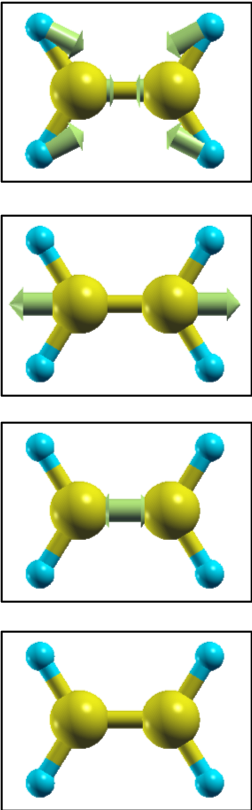
Finally, the vibrational modes and the corresponding zero-point energies
are calculated using program gif in directory ~/STATE/util/Vibration
$ ~/STATE/util/Vibration/src/gif < MD_2.data
.
.
.
Vibrational frequencies and eigen vectors
 NATM FAC       MODE  WR        : NU(meV)   NU(cm-1)
   7  0.10D+01  1      0.14D-04 :    2.37     19.09
        1   0.1666666636   0.0000000000  -0.0000321875
        2   0.0000000000   0.0000000000   0.0000000000
        3   0.0000000000   0.0000000000   0.0000000000
        4   0.0000000000   0.0000000000   0.0000000000
        5   0.0000000000   0.0000000000   0.0000000000
        6   0.0000000000   0.0000000000   0.0000000000
        7   0.0000000000   0.0000000000   0.0000000000
   7  0.10D+01  2      0.14D-04 :    2.37     19.09
        1   0.0000000000  -0.1666666667  -0.0000000000
        2   0.0000000000   0.0000000000   0.0000000000
        3   0.0000000000   0.0000000000   0.0000000000
        4   0.0000000000   0.0000000000   0.0000000000
        5   0.0000000000   0.0000000000   0.0000000000
        6   0.0000000000   0.0000000000   0.0000000000
        7   0.0000000000   0.0000000000   0.0000000000
   7  0.15D+00  3      0.36D-02 :   38.15    307.73
        1   0.0000321875  -0.0000000000   0.1666666636
        2   0.0000000000   0.0000000000   0.0000000000
        3   0.0000000000   0.0000000000   0.0000000000
        4   0.0000000000   0.0000000000   0.0000000000
        5   0.0000000000   0.0000000000   0.0000000000
        6   0.0000000000   0.0000000000   0.0000000000
        7   0.0000000000   0.0000000000   0.0000000000

              =======
              SUMMARY
              =======
 MODE  WR       : NU(meV)  NU(cm-1)
    1  0.14D-04 :    2.37     19.09
    2  0.14D-04 :    2.37     19.09
    3  0.36D-02 :   38.15    307.73
Similar analyses can be done in directories bridge
.
.
.
 Vibrational frequencies and eigen vectors
 NATM FAC       MODE  WR        : NU(meV)   NU(cm-1)
   7  0.10D+01  1      0.15D-03 :    7.78     62.73
        1   0.1178489705  -0.1178532500  -0.0000970020
        2   0.0000000000   0.0000000000   0.0000000000
        3   0.0000000000   0.0000000000   0.0000000000
        4   0.0000000000   0.0000000000   0.0000000000
        5   0.0000000000   0.0000000000   0.0000000000
        6   0.0000000000   0.0000000000   0.0000000000
        7   0.0000000000   0.0000000000   0.0000000000
   7  0.10D+01  2      0.24D-03 :    9.93     80.08
        1   0.1178531952   0.1178486620   0.0003082383
        2   0.0000000000   0.0000000000   0.0000000000
        3   0.0000000000   0.0000000000   0.0000000000
        4   0.0000000000   0.0000000000   0.0000000000
        5   0.0000000000   0.0000000000   0.0000000000
        6   0.0000000000   0.0000000000   0.0000000000
        7   0.0000000000   0.0000000000   0.0000000000
   7  0.30D+00  3      0.18D-02 :   27.22    219.56
        1  -0.0001493719  -0.0002865454   0.1666663534
        2   0.0000000000   0.0000000000   0.0000000000
        3   0.0000000000   0.0000000000   0.0000000000
        4   0.0000000000   0.0000000000   0.0000000000
        5   0.0000000000   0.0000000000   0.0000000000
        6   0.0000000000   0.0000000000   0.0000000000
        7   0.0000000000   0.0000000000   0.0000000000

              =======
              SUMMARY
              =======
 MODE  WR       : NU(meV)  NU(cm-1)
    1  0.15D-03 :    7.78     62.73
    2  0.24D-03 :    9.93     80.08
    3  0.18D-02 :   27.22    219.56
and hollow:
.
.
.
 Vibrational frequencies and eigen vectors
 NATM FAC       MODE  WR        : NU(meV)   NU(cm-1)
   7  0.10D+01  1     -0.36D-03 :   12.02     96.96
        1  -0.1178511111   0.1178511111   0.0000949646
        2   0.0000000000   0.0000000000   0.0000000000
        3   0.0000000000   0.0000000000   0.0000000000
        4   0.0000000000   0.0000000000   0.0000000000
        5   0.0000000000   0.0000000000   0.0000000000
        6   0.0000000000   0.0000000000   0.0000000000
        7   0.0000000000   0.0000000000   0.0000000000
   7  0.10D+01  2     -0.36D-03 :   12.02     96.96
        1   0.1178511302   0.1178511302   0.0000000000
        2   0.0000000000   0.0000000000   0.0000000000
        3   0.0000000000   0.0000000000   0.0000000000
        4   0.0000000000   0.0000000000   0.0000000000
        5   0.0000000000   0.0000000000   0.0000000000
        6   0.0000000000   0.0000000000   0.0000000000
        7   0.0000000000   0.0000000000   0.0000000000
   7  0.41D+00  3      0.14D-02 :   23.46    189.25
        1   0.0000671501  -0.0000671501   0.1666666396
        2   0.0000000000   0.0000000000   0.0000000000
        3   0.0000000000   0.0000000000   0.0000000000
        4   0.0000000000   0.0000000000   0.0000000000
        5   0.0000000000   0.0000000000   0.0000000000
        6   0.0000000000   0.0000000000   0.0000000000
        7   0.0000000000   0.0000000000   0.0000000000

              =======
              SUMMARY
              =======
 MODE  WR       : NU(meV)  NU(cm-1)
    1 -0.36D-03 :   12.02     96.96
    2 -0.36D-03 :   12.02     96.96
    3  0.14D-02 :   23.46    189.25